Page 36 - Computational Colour Science Using MATLAB

COMPUTING THE TRANSPOSE AND INVERSE OF MATRICES 23
only be used to invert matrices that are square. For non-square matrices
MATLAB provides the pinv command that computes a pseudoinverse. Whereas
1
the inverse of a matrix A is denoted by the symbol A , the pseudoinverse is
+
denoted by the symbol A .
However, it is usually more efficient and accurate (Borse, 1997) to solve
systems of simultaneous equations using Gaussian elimination or, equivalently,
by using MATLAB’s backslash division. Thus Equation (2.2) may be solved as
follows:

x = M\p;

The backslash operator is used extensively throughout this book for computing
the pseudoinverse of non-square matrices (a common mistake is to confuse the
backslash operator with the forwardslash operator which MATLAB uses to
divide one matrix by another).
For many matrices the inv and pinv commands will generate identical results to
the backslash operator. However, in some circumstances the matrix is ill-
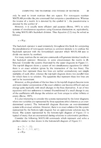
behaved. Consider the systems illustrated by the upper diagrams in Figure 3.1.
The top-left diagram shows a system of two simultaneous equations for which
there is an exact solution (given by the intersection of the two lines). The
equations that represent these two lines are neither contradictory nor simple
multiples of each other, whereas the top-right diagram shows two parallel lines
for which there is no solution. The equations that represent these two lines are
said to be inconsistent.
However, as the gradients of the two lines in the top-left diagram become more
and more similar computation of the exact solution can become difficult and can
change quite markedly with small changes in the lines themselves. A set of two
equations with two unknowns is termed ill-conditioned if a small change in any
of the coefficients will change the solution set from unique to either infinite or
empty (Borse, 1997).
It is also interesting to consider the systems represented by the lower diagrams
where two variables are represented by three equations (this is known as an over-
determined system). The bottom-left diagram illustrates an over-determined
system with an exact solution. However, there is no exact solution for the system
represented by the bottom-right diagram but an approximate solution may be
found. The system represented by the bottom-right diagram of Figure 3.1 is
typical of many that are encountered during solutions to colorimetric problems.
Consider the following MATLAB commands which represent and solve a
problem similar to that shown in the bottom-left diagram of Figure 3.1:

a = [1; 1; 2];
M = [1 -1; 1 1; 6 1];
x = M\a