Page 37 - Computational Colour Science Using MATLAB

24 A SHORT INTRODUCTION TO MATLAB

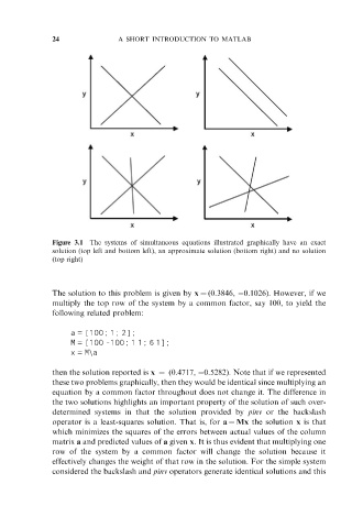
Figure 3.1 The systems of simultaneous equations illustrated graphically have an exact
solution (top left and bottom left), an approximate solution (bottom right) and no solution
(top right)

The solution to this problem is given by x ¼ (0.3846, 0.1026). However, if we
multiply the top row of the system by a common factor, say 100, to yield the
following related problem:

a = [100; 1; 2];
M = [100 -100; 1 1; 6 1];
x = M\a

then the solution reported is x ¼ (0.4717, 0.5282). Note that if we represented
these two problems graphically, then they would be identical since multiplying an
equation by a common factor throughout does not change it. The difference in
the two solutions highlights an important property of the solution of such over-
determined systems in that the solution provided by pinv or the backslash
operator is a least-squares solution. That is, for a ¼ Mx the solution x is that
which minimizes the squares of the errors between actual values of the column
matrix a and predicted values of a given x. It is thus evident that multiplying one
row of the system by a common factor will change the solution because it
effectively changes the weight of that row in the solution. For the simple system
considered the backslash and pinv operators generate identical solutions and this