Page 42 - Computational Colour Science Using MATLAB

INTERPOLATION METHODS 29
truncated, the CIE recommends the use of interpolation and extrapolation,
respectively (CIE, 1986b).

4.3 Interpolation methods

If reflectance data are available at 5-nm intervals, then the most accurate method
to compute tristimulus values is to use the 5-nm colour-matching and illuminant
data. Even if reflectance data are available at 10- or 20-nm intervals the 5-nm
data can be used if interpolation methods are applied to the reflectance data.
Another situation where interpolation methods may be important is where a user
is computing tristimulus values for a specific non-CIE illuminant. A problem
that the CIE has so far failed to solve is the disparity between illuminant spectral
power distributions and light sources that serve to correspond to these
illuminants. This is a particular problem with CIE illuminant D65, where
although there are many lamps that are used as D65 simulators there is, in fact,
no light source that replicates illuminant D65 exactly (Xu et al., 2003). A
practical solution to this problem is to measure the spectral power distribution of
the actual light source used in a specific viewing cabinet, for example, and to use
these measurements as the illuminant data in the colorimetric equations
[Equation (4.2)]. This approach is sensible; unfortunately many commercial
spectroradiometers provide radiance measurements at wavelength intervals of 4,
5 or 10 nm. Interpolation methods may be necessary to obtain the illuminant
data at 5-nm intervals. Interpolation methods are now briefly discussed before
alternative methods for computing tristimulus values are described.
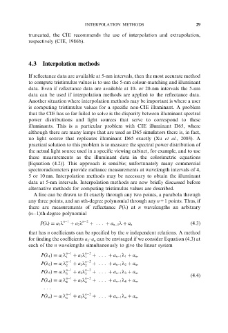
A line can be drawn to fit exactly through any two points, a parabola through
any three points, and an nth-degree polynomial through any n+1 points. Thus, if
there are measurements of reflectance P(l)at n wavelengths an arbitrary
(n 1)th-degree polynomial
n 1 n 2
þ ::: þ a n 1 l þ a n
PðlÞ¼ a 1 l þ a 2 l ð4:3Þ
that has n coefficients can be specified by the n independent relations. A method
for finding the coefficients a –a can be envisaged if we consider Equation (4.3) at
n
1
each of the n wavelengths simultaneously to give the linear system
n 1 n 2
Pðl 1 Þ¼ a 1 l 1 þ a 2 l 1 þ :: : þ a n 1 l 1 þ a n ,
n 1 n 2
2 2
Pðl 2 Þ¼ a 1 l þ a 2 l þ :: : þ a n 1 l 2 þ a n ,
n 1 n 2
Pðl 3 Þ¼ a 1 l 3 þ a 2 l 3 þ :: : þ a n 1 l 3 þ a n ,
n 1 n 2 ð4:4Þ
Pðl 4 Þ¼ a 1 l 4 þ a 2 l 4 þ :: : þ a n 1 l 4 þ a n ,
:: :
n 1 n 2
Pðl n Þ¼ a 1 l n þ a 2 l n þ :: : þ a n 1 l n þ a n ,