Page 45 - Computational Colour Science Using MATLAB

32 COMPUTING CIE TRISTIMULUS VALUES

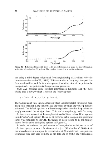
Figure 4.2 Polynomial fits (solid lines) to 20-nm reflectance data using the interp1 function
and cubic (a) and spline (b) options. The original data ( *) were at 10-nm intervals

out using a third-degree polynomial from neighbouring data within twice the
measurement interval (CIE, 1986b). This means that a Langrange interpolation
formula should be used for four data points (two either side of the point to be
interpolated). Interpolation is thus performed piecewise.
MATLAB provides some excellent interpolation functions and the most
widely used is interp1 which is used in the following way:

p = interp1(x,y,x1,<option>);

The vectors x and y are the data through which the interpolated curve must pass.
The points specified in the vector x1 are the points at which the vector p must be
estimated. The default option is a linear interpolation in which the y points are
simply connected by straight lines. This works surprisingly well for many
reflectance curves given that the sampling interval is 20 nm or less. Other options
include ‘cubic’ and ‘spline’. The cubic fit performs cubic interpolation piecemeal
in the way stipulated by the CIE. The results of interpolation to 20-nm data are
shown for the cubic and spline options in Figure 4.2.
In order to evaluate the performance of interpolation techniques a set of
reflectance spectra measured for 404 natural objects (Westland et al., 2000) at 10-
nm intervals were sub-sampled to generate data at 20-nm intervals. Interpolation
techniques were then used to fit the 20-nm data and to predict the reflectance at