Page 44 - Computational Colour Science Using MATLAB

INTERPOLATION METHODS 31

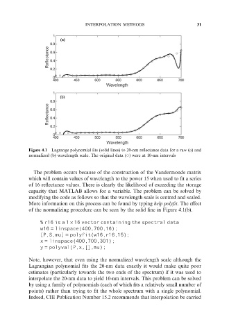
Figure 4.1 Lagrange polynomial fits (solid lines) to 20-nm reflectance data for a raw (a) and
normalized (b) wavelength scale. The original data ( *) were at 10-nm intervals

The problem occurs because of the construction of the Vandermonde matrix
which will contain values of wavelength to the power 15 when used to fit a series
of 16 reflectance values. There is clearly the likelihood of exceeding the storage
capacity that MATLAB allows for a variable. The problem can be solved by
modifying the code as follows so that the wavelength scale is centred and scaled.
More information on this process can be found by typing help polyfit. The effect
of the normalizing procedure can be seen by the solid line in Figure 4.1(b).

% r16 is a 1616 vector containing the spectral data
w16 = linspace(400,700,16);
[P,S,mu] = polyfit(w16,r16,15);
x = linspace(400,700,301);
y = polyval(P,x,[],mu);

Note, however, that even using the normalized wavelength scale although the
Lagrangian polynomial fits the 20-nm data exactly it would make quite poor
estimates (particularly towards the two ends of the spectrum) if it was used to
interpolate the 20-nm data to yield 10-nm intervals. This problem can be solved
by using a family of polynomials (each of which fits a relatively small number of
points) rather than trying to fit the whole spectrum with a single polynomial.
Indeed, CIE Publication Number 15.2 recommends that interpolation be carried