Page 43 - Computational Colour Science Using MATLAB

30 COMPUTING CIE TRISTIMULUS VALUES
which represents n simultaneous equations and n unknowns. In terms of linear
algebra (see Chapter 2) Equations (4.4) can be efficiently represented by
Equation (4.5):
p ¼ Ma, ð4:5Þ

where p is an n61 column matrix of reflectance values, a is an n61 column
matrix containing the coefficients a –a and M is a special n6n matrix known as
n
1
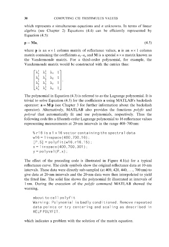
the Vandermonde matrix. For a third-order polynomial, for example, the
Vandermonde matrix would be constructed with the entries thus:
3 2
2 3
l 1 l 1 l 1 1
3 2
6 7
7.
l 2 l 2 l 2
6 1 7
6 3 2
4 l 3
l 3 l 3 1 5
3 2
l 4 l 4 l 4 1
The polynomial in Equation (4.3) is referred to as the Lagrange polynomial. It is
trivial to solve Equation (4.5) for the coefficients a using MATLAB’s backslash
operator: a ¼ M\p (see Chapter 3 for further information about the backslash
operator). Alternatively, MATLAB also provides the functions polyfit and
polyval that automatically fit and use polynomials, respectively. Thus the
following code fits a fifteenth-order Lagrange polynomial to 16 reflectance values
representing measurements at 20-nm intervals in the range 400–700 nm:

% r16 is a 1616 vector containing the spectral data
w16 = linspace(400,700,16);
[P,S] = polyfit(w16,r16,15);
x = linspace(400,700,301);
y = polyval(P,x);

The effect of the preceding code is illustrated in Figure 4.1(a) for a typical
reflectance curve. The circle symbols show the original reflectance data at 10-nm
intervals. These data were directly sub-sampled (at 400, 420, 440, . . ., 700 nm) to
give data at 20-nm intervals and the 20-nm data were then interpolated to yield
the fitted line. The solid line shows the polynomial fit illustrated at intervals of
1 nm. During the execution of the polyfit command MATLAB showed the
warning,

about to call polyfit
Warning: Polynomial is badly conditioned. Remove repeated
data points or try centering and scaling as described in
HELP POLYFIT.

which indicates a problem with the solution of the matrix equation.