Page 46 - Computational Colour Science Using MATLAB

EXTRAPOLATION METHODS 33
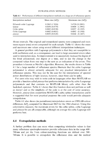
Table 4.1 Performance of different interpolation methods on a large set of reflectance spectra

Interpolation method Mean rms (DE* ab ) Maximum rms (DE* ab )

Fifteenth order Lagrange 0.2865 (1.7454) 3.4720 (18.3091)
Linear 0.0198 (0.4779) 0.0600 (1.3991)
Cubic spline 0.0082 (0.0330) 0.0297 (0.1305)
Cubic Lagrange 0.0002 (0.0051) 0.0092 (0.1508)
pinterp 0.0050 (0.0128) 0.0244 (0.1487)

10-nm intervals. The original and interpolated spectra were compared and root-
mean-square (rms) errors computed for each sample. Table 4.1 shows the mean
and maximum rms values using several different interpolation techniques.
A general problem with Lagrange polynomials is that they are susceptible to
wild oscillations and, as a consequence, can lead to large associated errors when
used to interpolate data. An improvement is to successively increase the degree of
the fitted polynomial, one degree at a time, and to use the change in the
computed values from one step to the next as an indication of the errors. This
procedure is known as Neville’s algorithm. However, the results shown in Table
4.1 for a large number of reflectance spectra illustrate that the cubic Lagrange
polynomial is almost certainly adequate for any practical interpolation of
reflectance spectra. This may not be the case for the interpolation of spectral
power distributions of light sources, however, since these can be spiky.
For users who may wish to write code in languages other than MATLAB we
provide a function called pinterp that performs interpolation by cubic Langrange
polynomials and that contains no MATLAB library calls other than the
backslash operator. Table 4.1 shows that this function does not perform as well
as interp1 and so the simplicity of the code is at the cost of some accuracy.
However, pinterp does outperform MATLAB’s cubic spline interpolation and it
is suggested that for most practical purposes the code would provide adequate
interpolation.
Table 4.1 also shows (in parentheses) interpolation errors as CIELAB colour
differences DE* computed for illuminant D65 for the 1964 observer. Using this
ab
colorimetric measure, the maximum errors for the cubic spline, cubic Lagrange
and pinterp fits are all comparable, although on average the cubic Lagrange still
performs best.

4.4 Extrapolation methods

A further problem that can occur when computing tristimulus values is that
many reflectance spectrophotometers provide reflectance data in the range 400–
700 nm and yet the 5-nm colour-matching functions are defined over 380–
780 nm. It is possible to extrapolate the reflectance data and the method