Page 293 - Computational Fluid Dynamics for Engineers

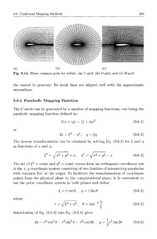
9.6 Conformal Mapping Methods 283

(a) (b) (c)
Fig. 9.14. Three common grids for airfoils, (a) C-grid, (b) O-grid, and (c) H-grid.

the easiest to generate. Its mesh lines are aligned well with the approximate
streamlines.

9.6.1 Parabolic Mapping Function

The C-mesh can be generated by a number of mapping functions, one being the
parabolic mapping function defined by:

2(x + iy) = (£ + n?) 2 (9.6.1)

or
2
2x = e-V , y = tr) (9.6.2)
The inverse transformation can be obtained by solving Eq. (9.6.2) for £ and 77
as functions of x and y,

£ 2 = \fx 2 + y 2 + x, rj 2 = \jx 2 + y 2 - x (9.6.3)

The set of £ 2 = const and rj 2 = const curves form an orthogonal curvilinear net
in the x, y coordinate system consisting of two families of intersecting parabolas
with common foci at the origin. To facilitate the transformation of coordinate
points from the physical plane to the computational plane, it is convenient to
use the polar coordinate system in both planes and define

£ = r cos 0, r] = r sin 9 (9.6.4)

where
2
t
r = y ^ + r? , 9 = a n - 1 ^ (9.6.5)
Substitution of Eq. (9.6.4) into Eq. (9.6.1) gives

2
2x = r 2 cos 9-r 2 sin 2 9 = r 2 cos 26>, y = -r 2 sin 29 (9.6.6)