Page 296 - Computational Fluid Dynamics for Engineers

286 9. Grid Generation

V\%VX\ViVVVy%tV%VVM\NVV%VV^ \vVVVVXVVXVVNVVyXVXVVNVVXVN^NVM.
(y = +*)
(ri=D
B _
E x
(ln2,0)
r H ,6 (n = 0) L
F
mUUlUVUVUmmUVUlUmUlUU TFWTOTW
(a) (b)

(c) (d)
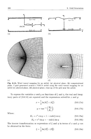
Fig. 9.15. Wind tunnel mapping for an airfoil: (a) physical plane, (b) computational
plane. C-grid generated around a NACA airfoil using the wind tunnel mapping for an
airfoil (c) physical plane, (d) physical plane, close-up of the grid near the airfoil.

To express the variables x and y as functions of £ and 77, the real and imag-
inary parts of (9.6.14) are equated and the expressions solved for x and y:
1
x=-]n(Kf + Ki) (9.6.17a)

K2
y = tan (9.6.17b)
Ki
Where:
K\ — e cos y — 1 — cosh £ cos 77 (9.6.18a)
K2 — e x sin y — — sinh £ sin 77 (9.6.18b)
The inverse transformation or expressions of £ and rj in terms of x and y can
be obtained in the form:
£ = - l n ( D § + L>|) (9.6.19a)