
Page 323 - Computational Fluid Dynamics for Engineers
P. 323
10.10 Model Problem for the MacCormack Method: Unsteady Shock Tube 313
not. In fact, it will be shown in Problem P10.4 that the first procedure is best
suited for discontinuities moving in the — x direction, while the second approach
is best suited for discontinuities moving in the +x direction. It can be seen that
a numerical boundary scheme is necessary on one side of the predictor step,
while a numerical boundary scheme is necessary on the opposite side on the
corrector step. This is true for both forward-backward and backward-forward
procedures described above.
10.10 Model Problem for the MacCormack Method:
Unsteady Shock Tube
To demonstrate the solution of the Euler equation for a one-dimensional com-
pressible flow with the MacCormack method, the model problem of a unsteady
shock tube is used as shown in Fig. 10.12.
Diaphragm
P P
\ J 5
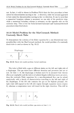
Fig. 10.12. Shock tube model problem: Initial conditions.
The tube is filled with a gas at different states on the left and right side of
a diaphragm. The gas states have different densities and pressures and are at
rest. At time t = 0, the diaphragm is broken and if it is assumed that viscous
effects are negligible and the tube is of infinite length (reflection waves are zero),
then the unsteady Euler equations for a one-dimensional flow can be solved
analytically with a family of characteristics travelling to the left and right of
the diaphragm. If the left side contains the gas at the highest pressure, the
right state will expand in the left side region through expansion waves (region
2), whereas a compression wave will travel in the right direction. This will be
1
p 3 | 4 P
l 5
1
2
Fig. 10.13. Shock tube model problem: gas states at time t > 0.