Page 335 - Computational Fluid Dynamics for Engineers

10.14 Model Problem for the Implicit Method: Quasi-ID Nozzle 325

2r-
Implicit CFL = 1.0 e e=10 1.75 t-
1.5F-
1.25 t--
s if.

0.75F-
0.5P-
0.25 P lmplicitCFL=1.0e e=10
i I i i i i I i i i i I i
Iterations x
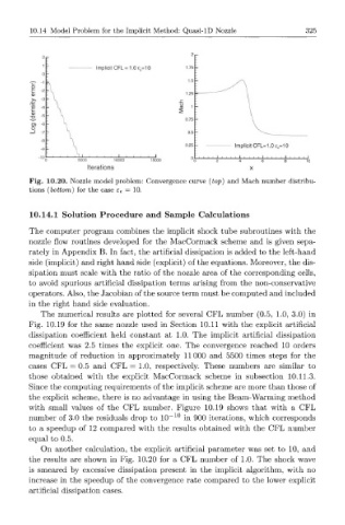
Fig. 10.20. Nozzle model problem: Convergence curve (top) and Mach number distribu-
tions (bottom) for the case e e = 10.

10.14.1 Solution Procedure and Sample Calculations
The computer program combines the implicit shock tube subroutines with the
nozzle flow routines developed for the MacCormack scheme and is given sepa-
rately in Appendix B. In fact, the artificial dissipation is added to the left-hand
side (implicit) and right hand side (explicit) of the equations. Moreover, the dis-
sipation must scale with the ratio of the nozzle area of the corresponding cells,
to avoid spurious artificial dissipation terms arising from the non-conservative
operators. Also, the Jacobian of the source term must be computed and included
in the right hand side evaluation.
The numerical results are plotted for several CFL number (0.5, 1.0, 3.0) in
Fig. 10.19 for the same nozzle used in Section 10.11 with the explicit artificial
dissipation coefficient held constant at 1.0. The implicit artificial dissipation
coefficient was 2.5 times the explicit one. The convergence reached 10 orders
magnitude of reduction in approximately 11000 and 5500 times steps for the
cases CFL = 0.5 and CFL = 1.0, respectively. These numbers are similar to
those obtained with the explicit MacCormack scheme in subsection 10.11.3.
Since the computing requirements of the implicit scheme are more than those of
the explicit scheme, there is no advantage in using the Beam-Warming method
with small values of the CFL number. Figure 10.19 shows that with a CFL
- 1 0
number of 3.0 the residuals drop to 10 in 900 iterations, which corresponds
to a speedup of 12 compared with the results obtained with the CFL number
equal to 0.5.
On another calculation, the explicit artificial parameter was set to 10, and
the results are shown in Fig. 10.20 for a CFL number of 1.0. The shock wave
is smeared by excessive dissipation present in the implicit algorithm, with no
increase in the speedup of the convergence rate compared to the lower explicit
artificial dissipation cases.