Page 67 - Computational Fluid Dynamics for Engineers

52 2. Conservation Equations

the grid spacing in the curvilinear space is uniform and of unit length, that is
Arj = 1, Z\£ = 1. This produces a computational space £,r/ with a rectangular
domain and with a regular uniform mesh so that, as we shall see in Section 6.3,
the differencing schemes used in the numerical formulation are simpler. The
original Cartesian space is usually referred to as the physical domain.
Using the chain rule of differential calculus, we can write

d _ d <9 <9£ d drj d d . d
~di = lh + dZ~di ^Fq'di
d d d£ d dri d _ d
— — - H = —ix H Vx (2.2.35)
dx dt; dx drj dx <9£ drj
d_ _ d_d^ JL^R-J^c A
dy ~ d£dy + dr)dy~ dC y + dr} Vy
or in compact form as
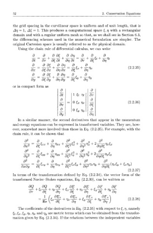
d d
dt 1 6 Vt\ dr
d d
= 0 £x Vx\ (2.2.36)
dx
d 0 Sy Vy\ d
dy 1 drj
In a similar manner, the second derivatives that appear in the momentum
and energy equations can be expressed in transformed variables. They are, how-
ever, somewhat more involved than those in Eq. (2.2.35). For example, with the
chain rule, it can be shown that

d 2 d 0 d 2 d 2 d 2
v_c2
o/-9Sx
dx 2 d^' xx + QiV. ] XX I d^ x ' ' dr, 271x + 2 drjd£, Vx<,x
d_ d_ & 2 &_ 2 0 d 2
dj]
dy 2 d^yy > nyy . ^ 2 s j , • Qr)2 drjd£
drj
d 2 d d d 2 d 2 d 2
71
dxdy d^ xy + drj ^ + ap^ v + d7] 2r]xJ]v + dridt (Vx£y + ixVy)
(2.2.37)
In terms of the transformation defined by Eq. (2.2.34), the vector form of the
transformed Navier-Stokes equations, Eq. (2.2.30), can be written as
dQ dQ dQ dE dE f dF dF

i dE v dE v dF v dF v (2.2.38)
Re Vx-?rr+ty-^-+Vy dr]
di
drj
The coefficients of the derivatives in Eq. (2.2.35) with respect to £, 77, namely
£,t,£,x,£,y,Vt, Vx and f] y are metric terms which can be obtained from the transfor-
mation given by Eq. (2.2.34). If the relations between the independent variables