Page 68 - Computational Fluid Dynamics for Engineers

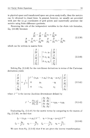
2.2 Navier-Stokes Equations 53

in physical space and transformed space are given analytically, then the metrics
can be obtained in closed form. In general, however, we usually are provided
with just the (x, y) coordinates of grid points and numerically generate the
metrics using finite-difference quotients.
Reversing the role of the independent variables in the chain rule formulas,
Eq. (2.2.36) becomes

d_ d_ d_ d_
dr dt dx dy (2.2.39)
d d d d d d_
v Vr]
<9£ dx ^ dy ^ dr] dx dy
which can be written in matrix form

d_ d_
dr 1 x T y T dt
d_ d_
0 xt yz (2.2.40)
dx
d_ u XJJ y^ d_
dr] dy

Solving Eq. (2.2.40) for the curvilinear derivatives in terms of the Cartesian
derivatives yields

d d_
1
dt J {xr,y T - x Ty v) (x Ty^ - y Tx^) dr
d 1 d_
0 y v -ys (2.2.41)
dx di
d 0 x e d_
dy dt]
1
where J is the inverse Jacobian determinant defined by
dx dy
-i _ d(x,y) _ dt, dt
x
J- X£Vv - nV£. (2.2.42)
d($,V) dx dy
dr] dr]
Evaluating Eq. (2.2.41) for the metric terms by comparing to the matrix of
Eq. (2.2.36), we find that

it = (X^VT ~ x Ty v)/J 1 , rjt = (x Ty£ - y Tx^)/J 1
(2.2.43)
Jhj_ J/|_
& Vx = 1 Zv = - % = 1
J" J -
We note from Eq. (2.2.43) that if we are given the inverse transformation