Page 73 - Computational Fluid Dynamics for Engineers

58 2. Conservation Equations

simplified further by retaining only the viscous and heat transfer terms with
derivatives in the coordinate direction normal to the body surface y or, for free
shear flows, the direction normal to the thin layer. This is referred to as the
thin-layer Navier-Stokes approximation and leads to the following equations
for three-dimensional flows with the continuity equation remaining unaltered:

2
du du du dp d u d —;—,
Qu— + Qv^- + QW— = - — + ii—-x - Q—U'V' + gf x (2.4.4)
z
dx oy oz dz ox dx oy oy
dv dv dv dp d\ d-*
QU— + gv— + gw — 2 72 + efv (2.4.5)
ox oy oz dy dy dy
2
dw dw dw dp d w d
f
QU — + QV — + QW — 2 Q — V W f • Qfz (2.4.6)
ox oy oz dz dy
dy
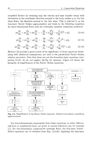
Blottner [8] provides a good review of the significance of these equations which,
along with additional assumptions, are used in the parabolized Navier-Stokes
solution procedure. Note that these are not the boundary-layer equations (sub-
section 2.4.3): we do not neglect dp/dy, for instance. Figure 2.2 shows the
hierarchy of simplification of the Navier-Stokes equations.

Full time-dependent
Navier-Stokes Eqs. Acceleration » 0
T
dS/dx« 1
(Time) Average
(Timi
Average small eddies V-Q
tvera
only j Stokes Eqs.
Reynolds-averaged
Navier-Stokes eqs. i
(turbulent flow)
> Large-eddy
d8/dx« 1 : simulation EuJer
eqs. eqs.
Thin-layer or Thin-layer or parabolized
parabolized laminar turbulent Navier-Stokes eqs.
Navier-Stokes eqs. (turbulent flow) j - Irrotationai
I
dp dp ? 'dp_
Laplace
dy dz dy l\di . * eq.
jh
Laminar Turbulent
boundary-layer boundary-layer
eqjs. eqs,
Fig. 2.2. Simplification of the Navier-Stokes equations. Dashed boxes denote simplifying
approximations.

For three-dimensional compressible flows these equations, in either differen-
tial form or transformed form, are given in several references (see for example
[1]). For two-dimensional compressible unsteady flows, the thin-layer Navier-
Stokes equations can be obtained from Eqs. (2.2.45). Applying the thin-layer