Page 84 - Computational Fluid Dynamics for Engineers

2.6 Classification of Conservation Equations 69

NO REAL

(a) (b) (c)
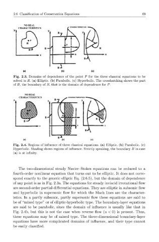
Fig. 2.3. Domains of dependence of the point P for the three classical equations to be
solved in R. (a) Elliptic, (b) Parabolic, (c) Hyperbolic. The crosshatching shows the part
of B, the boundary of R, that is the domain of dependence for P.

(a) (b) (c)
Fig. 2.4. Regions of influence of three classical equations, (a) Elliptic, (b) Parabolic, (c)
Hyperbolic. Shading shows regions of influence. Strictly speaking, the boundary B in case
(a) is at infinity.

The two-dimensional steady Navier-Stokes equations can be reduced to a
fourth-order nonlinear equation that turns out to be elliptic. It does not corre-
spond exactly to the generic elliptic Eq. (2.6.5), but the domain of dependence
of any point is as in Fig. 2.3a. The equations for steady inviscid irrotational flow
are second-order partial-differential equations. They are elliptic in subsonic flow
and hyperbolic in supersonic flow for which the Mach lines are the character-
istics. In a partly subsonic, partly supersonic flow these equations are said to
be of "mixed type" or of elliptic-hyperbolic type. The boundary-layer equations
are said to be parabolic, since the domain of influence is usually like that in
Fig. 2.4b, but this is not the case when reverse flow (u < 0) is present. Thus,
these equations may be of mixed type. The three-dimensional boundary-layer
equations have more complicated domains of influence, and their type cannot
be easily classified.