Page 26 - Computational Modeling in Biomedical Engineering and Medical Physics

12 Computational Modeling in Biomedical Engineering and Medical Physics

known. In inverse problems, either the structure of the system, or the materials and
their properties, or the sources are unknown. In fact they make the object of the anal-
ysis. Examples of inverse problems are the electrical potential cardiac mapping, the
ultrasound tomography, the thermography, the electrical impedance tomography, and
so on.
Inverse problems are usually ill-posed and their solutions may be constructed on
the “skeletons” produced by direct problems. For instance, in cardiac mapping the
transfer operator (e.g., a rectangular transfer matrix, in numerical simulation) that pro-
jects the electrical potential from the thorax surface onto the epicardium surface may
be obtained by solving a companion direct problem, which assumes the type of elec-
trical source (monopole, dipole) and its localization (Mocanu, 2002). The solution to
this problem requires the usage of inversion methods, singular value decomposition
based algorithms, regularization methods, and so on (Vetterling et al., 1997).
The direct problems of heat and mass transfer, electromagnetism, structural
mechanics and transport are frequently problems of equilibrium, eigenvalues,or transmis-
sion type.
Equilibrium problems are boundary value problems only. The physical quantities
are constant in time and the associated PDE is stationary, that is, there are no time
derivatives (Fig. 1.1). Examples of equilibrium problems are for instance the stationary
EMFs (electrostatic, magnetostatic, electrokinetic, stationary magnetic field), stationary
heat and mass (diffusion and/or convection) transfer, potential and stationary flows.
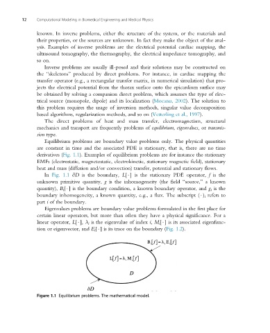
In Fig. 1.1 @D is the boundary, L[ ] is the stationary PDE operator, f is the
unknown primitive quantity, g is the inhomogeneity (the field “source,” a known
quantity), B i [ ] is the boundary condition, a known boundary operator, and g i is the
boundary inhomogeneity, a known quantity, e.g., a flux. The subscript ( ) i refers to
part i of the boundary.
Eigenvalues problems are boundary value problems formulated in the first place for
certain linear operators, but more than often they have a physical significance. For a
linear operator, L[ ], λ i is the eigenvalue of index i, M i [ ] is its associated eigenfunc-
tion or eigenvector, and E i [ ] is its trace on the boundary (Fig. 1.2).

Figure 1.1 Equilibrium problems. The mathematical model.