Page 27 - Computational Modeling in Biomedical Engineering and Medical Physics

Physical, mathematical, and numerical modeling 13

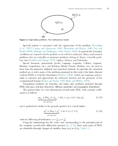
Figure 1.2 Eigenvalues problems. The mathematical model.

Spectral analysis is concerned with the eigensystem of the problem (Vetterling
et al., 1997; Canuto and Quateroni, 1984; Ehrenstein and Peyret, 1989; Fox and
Parker (1968); Morega and Nishimura, 1996; Peyret, 2002). In general the boundary
conditions are imposed and the problem to be solved is stationary. Many mathematical
problems that are reducible to stationary problems belong to Sturm Liouville prob-
lem class (Gottlieb and Orszag, 1977): Laplace, Poisson, and Helmholtz.
Special functions, polynomials (Jacobi, Lagrange, Legendre, Cebâ¸sev, Laguerre,
Hermite, Gegenbauer, etc.), and functions (Bessel, Fourier, Mathieu, etc.) are used to
form bases for projective analytical and numerical methods. In particular the numerical
method use to solve many of the problems presented in this work is the finite element
method (FEM) in Galerkin formulation Fletcher (1984), which uses Lagrange polyno-
mials to represent and approximate the unknown function and the geometry of the
computational domain (Peyret and Taylor, 1983; Bathe and Wilson, 1976).
Transmission problems are boundary and initial value problems presented through
PDEs with space and time derivatives: diffusion (parabolic) and propagation (hyperbolic).
The general form of a two-dimensional second-order PDE, with constant coeffi-
cients is as follows:

aφ 1 2bφ 1 cφ yy 1 dφ 1 eφ 1 f φ 5 gx; yÞ; ð1:15Þ
ð
x
xx
y
xy
|fflfflfflfflfflfflfflfflfflfflfflfflfflfflffl{zfflfflfflfflfflfflfflfflfflfflfflfflfflfflffl}
principal part
and is qualitatively similar to the general equation of a conical surface
2
2
ax 1 2bxy 1 cy 1 dx 1 ey 1 f 5 0; ð1:16Þ
|fflfflfflfflfflfflfflfflfflfflfflffl{zfflfflfflfflfflfflfflfflfflfflfflffl}
principal part
@
with the following identification: x2 @ ; y2 .
@x @y
Using the terminology for the conics and corresponding to the principal part of
the complete second-order differential operator Eq. (1.15), three main types of PDEs
are obtainable through changes of variables, from (x,y)to(ξ,η), Table 1.1.