Page 194 - Computational Statistics Handbook with MATLAB
P. 194

Chapter 5: Exploratory Data Analysis                            181


                             rotates. We believe that the extra dimension conveyed by the speed is difficult
                             to understand unless the analyst has experience looking at grand tour mov-
                             ies.
                              In order to implement the pseudo grand tour, we need a way of obtaining
                             the projection vectors α αα α t()   and β ββ β t()  . First we consider the data vector x. If d
                             is odd, then we augment each data point with a zero, to get an even number
                             of elements. In this case,

                                                x =  ( x … x 0,  ,  , );  for  d odd.
                                                      1    d
                             This will not affect the projection. So, without loss of generality, we present
                             the method with the understanding that d is even. We take the vector α αα α t()   to
                             be

                                                 ⁄
                                                                ,
                                                                   ,
                                                                           ,
                                        α α α α t() =  2 d sin(  ω t cos,  ω t … sin ω  d 2 t cos ω d 2 t)  ,  (5.24)
                                                                         ⁄
                                                                                  ⁄
                                                        1
                                                               1
                             and the vector β ββ β t()   as
                                                                ,
                                                                   ,
                                                ⁄
                                                                           ,
                                      β β β β t() =  2 d cos(  ω 1 t –,  sin ω 1 t … cos  ω d 2⁄ t – sin ω d 2⁄ t)  .  (5.25)
                              We  choose ω i  and ω j  such  that the  ratio ω ω⁄  j  is  irrational  for every  i and
                                                                    i
                             j. Additionally, we must choose these such that no  ω ω⁄   is a rational multi-
                                                                           i  j
                             ple of any other ratio. It is also recommended that the time step ∆t   be a small
                             positive irrational number. One way to obtain irrational values for ω   is to let
                                                                                        i
                             ω =   P  , where P   is the i-th prime number.
                              i     i         i
                              The steps for implementing the 2-D pseudo grand tour are given here. The
                             details on how to implement this in MATLAB are given in Example 5.28.
                             PROCEDURE - PSEUDO GRAND TOUR
                                              to an irrational number.
                                1. Set each  ω i
                                2. Find vectors  α αα α t()  and  β ββ β t()   using Equations 5.24 and 5.25.
                                3. Project the data onto the plane spanned  by  these vectors using
                                   Equations 5.23 and 5.24.
                                                              α α α α t()  β β β β t()
                                4. Display the projected points,  z i   and  z i  , in a 2-D scatterplot.
                                5.  Using  ∆t   irrational, increment  the time, and repeat steps 2
                                   through 4.

                             Before we illustrate this in an example, we note that once we stop the tour at
                             an interesting projection, we can easily recover the projection by knowing the
                             time step.


                            © 2002 by Chapman & Hall/CRC
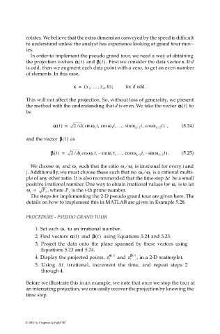
   189   190   191   192   193   194   195   196   197   198   199