Page 29 - Computational Statistics Handbook with MATLAB

Chapter 2: Probability Concepts 15

b
(
Pa ≤ X ≤ b) = ∫ fx()d . x (2.1)
a
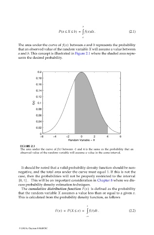
The area under the curve of f x() between a and b represents the probability
that an observed value of the random variable X will assume a value between
a and b. This concept is illustrated in Figure 2.1 where the shaded area repre-
sents the desired probability.

0.2
0.18

0.16
0.14
0.12
f(x) 0.1
0.08
0.06

0.04
0.02
0
−6 −4 −2 0 2 4 6
Random Variable − X

2.1
II
IG
F F FI F U URE GU 2.1 RE RE RE 2.1
GU
G
2.1
The area under the curve of f(x) between -1 and 4 is the same as the probability that an
observed value of the random variable will assume a value in the same interval.
It should be noted that a valid probability density function should be non-
negative, and the total area under the curve must equal 1. If this is not the
case, then the probabilities will not be properly restricted to the interval
[ 01] . This will be an important consideration in Chapter 8 where we dis-
,
cuss probability density estimation techniques.
The cumulative distribution function Fx() is defined as the probability
that the random variable X assumes a value less than or equal to a given x.
This is calculated from the probability density function, as follows

x
(
Fx() = PX ≤ x) = ∫ ft()d . t (2.2)
– ∞

© 2002 by Chapman & Hall/CRC