Page 39 - Computational Statistics Handbook with MATLAB

Chapter 2: Probability Concepts 25

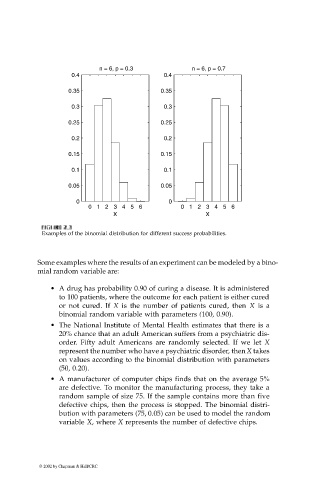
n = 6, p = 0.3 n = 6, p = 0.7
0.4 0.4

0.35 0.35

0.3 0.3

0.25 0.25

0.2 0.2
0.15 0.15

0.1 0.1

0.05 0.05
0 0
0 1 2 3 4 5 6 0 1 2 3 4 5 6
X X

FI F U URE G 2. RE 2. 3 3
IG
3
GU
F F II GU RE RE 2. 2. 3
Examples of the binomial distribution for different success probabilities.
Some examples where the results of an experiment can be modeled by a bino-
mial random variable are:

• A drug has probability 0.90 of curing a disease. It is administered
to 100 patients, where the outcome for each patient is either cured
or not cured. If X is the number of patients cured, then X is a
binomial random variable with parameters (100, 0.90).
• The National Institute of Mental Health estimates that there is a
20% chance that an adult American suffers from a psychiatric dis-
order. Fifty adult Americans are randomly selected. If we let X
represent the number who have a psychiatric disorder, then X takes
on values according to the binomial distribution with parameters
(50, 0.20).
• A manufacturer of computer chips finds that on the average 5%
are defective. To monitor the manufacturing process, they take a
random sample of size 75. If the sample contains more than five
defective chips, then the process is stopped. The binomial distri-
bution with parameters (75, 0.05) can be used to model the random
variable X, where X represents the number of defective chips.

© 2002 by Chapman & Hall/CRC