Page 44 - Computational Statistics Handbook with MATLAB

30 Computational Statistics Handbook with MATLAB

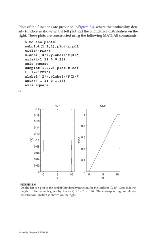
Plots of the functions are provided in Figure 2.4, where the probability den-
sity function is shown in the left plot and the cumulative distribution on the
right. These plots are constructed using the following MATLAB commands.
% Do the plots.
subplot(1,2,1),plot(x,pdf)
title('PDF')
xlabel('X'),ylabel('f(X)')
axis([-1 11 0 0.2])
axis square
subplot(1,2,2),plot(x,cdf)
title('CDF')
xlabel('X'),ylabel('F(X)')
axis([-1 11 0 1.1])
axis square

PDF CDF
0.2
0.18 1
0.16
0.8
0.14
0.12
f(X) 0.1 F(X) 0.6

0.08
0.4
0.06
0.04 0.2
0.02

0 0
0 5 10 0 5 10
X X

IG
FI F U URE G 2. RE 2. 4 4
GU
F F II GU RE RE 2. 2. 4
4
On the left is a plot of the probability density function for the uniform (0, 10). Note that the
⁄
height of the curve is given by 1 (⁄ b – a) = 110 = 0.10 . The corresponding cumulative
distribution function is shown on the right.

© 2002 by Chapman & Hall/CRC