Page 46 - Computational Statistics Handbook with MATLAB

32 Computational Statistics Handbook with MATLAB

Normal Distribution
1

0.9
µ = 2
0.8 σ = 0.5
0.7
0.6
f(x) 0.5 µ = 0
σ = 1
0.4
0.3 µ = − 2
σ = 2
0.2
0.1
0
−8 −6 −4 −2 0 2 4 6
X

GU
2.5
2.5
GU
F F FI F U URE G 2.5 RE RE RE 2.5
IG
II
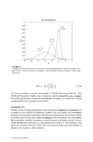
Examples of probability density functions for normally distributed random variables. Note
that as the variance increases, the height of the probability density function at the mean
decreases.
z
1  -------  1
-
Φ z() = --erf   + . -- - (2.32)
2  2  2
The error function can be calculated in MATLAB using erf(x). The
MATLAB Statistics Toolbox has a function called normcdf(x,mu,sigma)
that will calculate the cumulative distribution function for values in x. Its use
is illustrated in the example given below.

Example 2.5
Similar to the uniform distribution, the functions normpdf and normcdf are
available in the MATLAB Statistics Toolbox for calculating the probability
density function and cumulative distribution function for the normal. There
is another special function called normspec that determines the probability
that a random variable X assumes a value between two limits, where X is nor-
µ
mally distributed with mean and standard deviation σ. This function also
plots the normal density, where the area between the specified limits is
shaded. The syntax is shown below.

© 2002 by Chapman & Hall/CRC