Page 51 - Computational Statistics Handbook with MATLAB

Chapter 2: Probability Concepts 37

 0; x ≤ 0
,
(

;
Fx λ t) =  1 λx t – 1 – y (2.39)
∫
 ---------- y e d y; x > 0 .
Γ t()

0
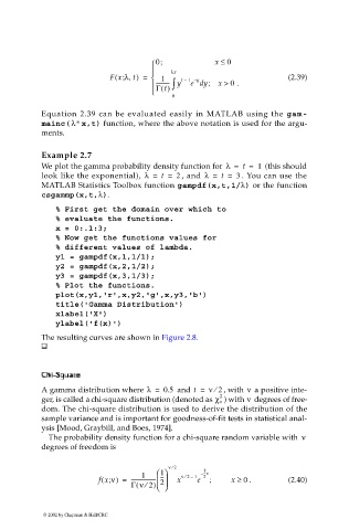
Equation 2.39 can be evaluated easily in MATLAB using the gam-
mainc(λ* x,t) function, where the above notation is used for the argu-
ments.
Example 2.7
We plot the gamma probability density function for λ = t = 1 (this should
look like the exponential), λ = t = 2 , and λ = t = 3 . You can use the
MATLAB Statistics Toolbox function gampdf(x,t,1/λ) or the function
csgammp(x,t,λ).
% First get the domain over which to
% evaluate the functions.
x = 0:.1:3;
% Now get the functions values for
% different values of lambda.
y1 = gampdf(x,1,1/1);
y2 = gampdf(x,2,1/2);
y3 = gampdf(x,3,1/3);
% Plot the functions.
plot(x,y1,'r',x,y2,'g',x,y3,'b')
title('Gamma Distribution')
xlabel('X')
ylabel('f(x)')
The resulting curves are shown in Figure 2.8.

Chi ChiChi Chi- -SSquarequare
-- SSquarequare
⁄
ν
A gamma distribution where λ = 0.5 and t = ν 2 , with a positive inte-
ν
2
ger, is called a chi-square distribution (denoted as χ ν ) with degrees of free-
dom. The chi-square distribution is used to derive the distribution of the
sample variance and is important for goodness-of-fit tests in statistical anal-
ysis [Mood, Graybill, and Boes, 1974].
The probability density function for a chi-square random variable with ν
degrees of freedom is
⁄
ν 2
1  – 1 --x
-
1
⁄
--
-
(
;
f x ν) = ------------------  x ν 2 – 1 e 2 ; x ≥ . 0 (2.40)
2
⁄
Γν 2) 
(
© 2002 by Chapman & Hall/CRC