Page 53 - Computational Statistics Handbook with MATLAB

Chapter 2: Probability Concepts 39

β
ν
  x –  -
ν
-----------
α 
β
x –
β –
1 –
--- 
,,
(
;
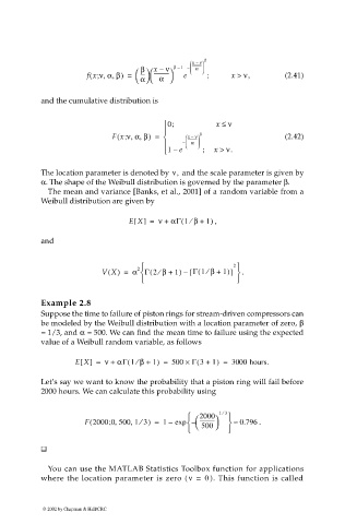
f x ν αβ) =  ------------ e   ; x > ν, (2.41)
α 
α 

and the cumulative distribution is
 0; x ≤ ν
(
,,

Fx ν αβ) =   x –  β (2.42)
ν
;
-----------
-
  –  α  
 1 – e ; x > ν.
The location parameter is denoted by ν, and the scale parameter is given by
α. The shape of the Weibull distribution is governed by the parameter β.
The mean and variance [Banks, et al., 2001] of a random variable from a
Weibull distribution are given by
(
⁄
EX[] = ν + αΓ 1 β + 1) ,
and
2  2 
(
⁄

VX() = α Γ 2 β⁄( + 1) – [ Γ 1 β + 1)] . 
 
Example 2.8
Suppose the time to failure of piston rings for stream-driven compressors can
be modeled by the Weibull distribution with a location parameter of zero, β
= 1/3, and α = 500. We can find the mean time to failure using the expected
value of a Weibull random variable, as follows
⁄
(
(
EX[] = ν + αΓ 1 β + 1) = 500 × Γ 3 + 1) = 3000 hours.
Let’s say we want to know the probability that a piston ring will fail before
2000 hours. We can calculate this probability using
⁄
  2000 13 
⁄
(
,
,
-
F 2000 0 500 1 3) = 1 – exp  –  -----------  ≈ 0.796 .
;
500 
 

You can use the MATLAB Statistics Toolbox function for applications
where the location parameter is zero ( ν = 0 ). This function is called

© 2002 by Chapman & Hall/CRC