Page 55 - Computational Statistics Handbook with MATLAB

Chapter 2: Probability Concepts 41

x
1
,
(
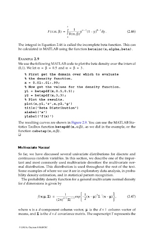
Fx α β) = ∫ ------------------y α – 1 ( 1 – y) β – 1 d . y (2.46)
;
B αβ)
(
,
0
The integral in Equation 2.46 is called the incomplete beta function. This can
be calculated in MATLAB using the function betainc(x,alpha,beta).
EXAMPLE 2.9
We use the following MATLAB code to plot the beta density over the interval
(0,1). We let α = β = 0.5 and α = β = 3 .
% First get the domain over which to evaluate
% the density function.
x = 0.01:.01:.99;
% Now get the values for the density function.
y1 = betapdf(x,0.5,0.5);
y2 = betapdf(x,3,3);
% Plot the results.
plot(x,y1,'r',x,y2,'g')
title('Beta Distribution')
xlabel('x')
ylabel('f(x)')
The resulting curves are shown in Figure 2.9. You can use the MATLAB Sta-
tistics Toolbox function betapdf(x,α,β), as we did in the example, or the
function csbetap(x,α,β).

r
o
rmma
Mult Multi MultMult ivvar vvarar ar i iaat aatt teeNNo a l l ll
NoNo
rr mama
ii
ii
ee
So far, we have discussed several univariate distributions for discrete and
continuous random variables. In this section, we describe one of the impor-
tant and most commonly used multivariate densities: the multivariate nor-
mal distribution. This distribution is used throughout the rest of the text.
Some examples of where we use it are in exploratory data analysis, in proba-
bility density estimation, and in statistical pattern recognition.
The probability density function for a general multivariate normal density
for d dimensions is given by
1
,
--- x –(
(
–
T
1

f x;µ µµ µΣ ΣΣ Σ) = -------------------------------exp  – 1 µ µ µ µ) Σ ( x – µ µ µ µ)  ,  (2.47)
⁄
⁄
( 2π) d 2 Σ Σ Σ Σ 12  2 
µ µ µ µ
where x is a d-component column vector, is the d × 1 column vector of
Σ Σ Σ Σ
means, and is the d × d covariance matrix. The superscript T represents the
© 2002 by Chapman & Hall/CRC