Page 54 - Computational Statistics Handbook with MATLAB

40 Computational Statistics Handbook with MATLAB

weibcdf (for the cumulative distribution function), and the input arguments
−β
−β
−β−β
are: (x,α αα α ,β). The reason for the different parameters is that MATLAB uses
an alternate definition for the Weibull probability density function given by
b
ax
1 –
,
(
b –
;
f xa b) = abx e ; x > . 0 (2.43)
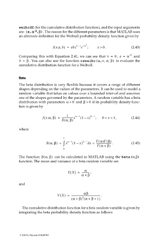
Comparing this with Equation 2.41, we can see that ν = 0 , a = α – β and
b = β . You can also use the function csweibc(x,ν, α, β) to evaluate the
cumulative distribution function for a Weibull.
aa
Be taa
BBeett
Bet
The beta distribution is very flexible because it covers a range of different
shapes depending on the values of the parameters. It can be used to model a
random variable that takes on values over a bounded interval and assumes
one of the shapes governed by the parameters. A random variable has a beta
distribution with parameters α > 0 and β > 0 if its probability density func-
tion is given by

1
,
(
f x α β) = ------------------x α – 1 ( 1 – x) β – 1 ; 0 < x < , 1 (2.44)
;
B αβ)
,
(
where
1
(
,
B αβ) = ∫ x α – 1 ( 1 – x) β – 1 d x = Γα()Γ β() . (2.45)
-------------------------
(
Γα + β)
0
The function B αβ,( ) can be calculated in MATLAB using the beta(α,β)
function. The mean and variance of a beta random variable are
α
EX[] = ------------- ,
α + β

and

αβ
VX() = ------------------------------------------------ .
2
( α + β) α +( β + 1)
The cumulative distribution function for a beta random variable is given by
integrating the beta probability density function as follows

© 2002 by Chapman & Hall/CRC