Page 49 - Computational Statistics Handbook with MATLAB

Chapter 2: Probability Concepts 35

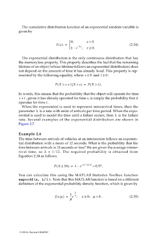
The cumulative distribution function of an exponential random variable is
given by

 0; x < 0
Fx() =  λx (2.34)
 1 – e – ; x ≥ 0.

The exponential distribution is the only continuous distribution that has
the memoryless property. This property describes the fact that the remaining
lifetime of an object (whose lifetime follows an exponential distribution) does
not depend on the amount of time it has already lived. This property is rep-
resented by the following equality, where s ≥ 0 and t ≥ : 0

PX > s + t X > s) = PX > t . )
(
(
In words, this means that the probability that the object will operate for time
s + t , given it has already operated for time s, is simply the probability that it
operates for time t.
When the exponential is used to represent interarrival times, then the
λ
parameter is a rate with units of arrivals per time period. When the expo-
λ
nential is used to model the time until a failure occurs, then is the failure
rate. Several examples of the exponential distribution are shown in
Figure 2.7.

Example 2.6
The time between arrivals of vehicles at an intersection follows an exponen-
tial distribution with a mean of 12 seconds. What is the probability that the
time between arrivals is 10 seconds or less? We are given the average interar-
⁄
rival time, so λ = 112 . The required probability is obtained from
Equation 2.34 as follows

⁄
(
PX ≤ 10) = 1 – e ( – 112)10 ≈ 0.57 .
You can calculate this using the MATLAB Statistics Toolbox function
λ
expocdf(x, 1/ ). Note that this MATLAB function is based on a different
definition of the exponential probability density function, which is given by

x ---
–
(
;
f x µ) = 1 µ x ≥ 0 µ > . 0 (2.35)
;
---e ;
µ

© 2002 by Chapman & Hall/CRC