Page 45 - Computational Statistics Handbook with MATLAB

Chapter 2: Probability Concepts 31

rmma
a
l
No
NNoorr mama ll l
Nor
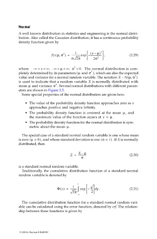
A well known distribution in statistics and engineering is the normal distri-
bution. Also called the Gaussian distribution, it has a continuous probability
density function given by
µ) 
2
x –
1
; ,
(
2

f x µ σ ) = --------------exp  – ( -------------------  , (2.29)
σ 2π  2σ 2 
where – ∞ < x < ∞ –; ∞ < µ < ∞ σ >; 2 0. The normal distribution is com-
pletely determined by its parameters ( and σ 2 ), which are also the expected
µ
(
,
value and variance for a normal random variable. The notation X ∼ N µσ )
2
is used to indicate that a random variable X is normally distributed with
mean and variance σ 2 . Several normal distributions with different param-
µ
eters are shown in Figure 2.5.
Some special properties of the normal distribution are given here.
• The value of the probability density function approaches zero as x
approaches positive and negative infinity.
• The probability density function is centered at the mean µ , and
the maximum value of the function occurs at x = µ .
• The probability density function for the normal distribution is sym-
µ
metric about the mean .
The special case of a standard normal random variable is one whose mean
is zero µ =( 0) , and whose standard deviation is one σ =( 1) . If X is normally
distributed, then

X – µ
Z = ------------- (2.30)
σ

is a standard normal random variable.
Traditionally, the cumulative distribution function of a standard normal
random variable is denoted by

z
2
1  y 
Φ z() = ---------- ∫ exp  – -----  d . y (2.31)
2π  2 
– ∞
The cumulative distribution function for a standard normal random vari-
able can be calculated using the error function, denoted by erf. The relation-
ship between these functions is given by

© 2002 by Chapman & Hall/CRC