Page 231 -

Section 7.1 Binocular Camera Geometry and the Epipolar Constraint 199

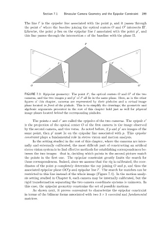
The line l is the epipolar line associated with the point p, and it passes through

the point e where the baseline joining the optical centers O and O intersects Π .
Likewise, the point p lies on the epipolar line l associated with the point p ,and

this line passes through the intersection e of the baseline with the plane Π.
P
’

p p’

l l’

e e’
O O’

FIGURE 7.3: Epipolar geometry: The point P,the opticalcenters O and O of the two

cameras, and the two images p and p of P all lie in the same plane. Here, as in the other
figures of this chapter, cameras are represented by their pinholes and a virtual image
plane located in front of the pinhole. This is to simplify the drawings; the geometric and
algebraic arguments presented in the rest of this chapter hold just as well for physical
image planes located behind the corresponding pinholes.

The points e and e are called the epipoles of the two cameras. The epipole e

is the projection of the optical center O of the first camera in the image observed
by the second camera, and vice versa. As noted before, if p and p are images of the

same point, then p must lie on the epipolar line associated with p. This epipolar
constraint plays a fundamental role in stereo vision and motion analysis.
In the setting studied in the rest of this chapter, where the cameras are inter-
nally and externally calibrated, the most difficult part of constructing an artifical
stereo vision system is to find effective methods for establishing correspondences be-
tween the two images—that is, deciding which points in the second picture match
the points in the first one. The epipolar constraint greatly limits the search for
these correspondences. Indeed, since we assume that the rig is calibrated, the coor-
dinates of the point p completely determine the ray joining O and p, and thus the

associated epipolar plane OO p and epipolar line l . The search for matches can be

restricted to this line instead of the whole image (Figure 7.4). In the motion analy-
sis setting studied in Chapter 8, each camera may be internally calibrated, but the
rigid transformation separating the two camera coordinate systems is unknown. In
this case, the epipolar geometry constrains the set of possible motions.
As shown next, it proves convenient to characterize the epipolar constraint
in terms of the bilinear forms associated with two 3 × 3 essential and fundamental
matrices.