Page 232 -

Section 7.1 Binocular Camera Geometry and the Epipolar Constraint 200

P
1 P
’
P
2
p p’
p’
1
p’
2
l l’
e e’
O O’

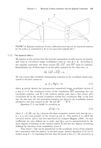
FIGURE 7.4: Epipolar constraint: Given a calibrated stereo rig, the set of possible matches

for the point p is constrained to lie on the associated epipolar line l .

7.1.2 The Essential Matrix

We assume in this section that the intrinsic parameters of each camera are known,
and work in normalized image coordinates—that is, take p = ˆ p. According to
−→ −−→ −−→
the epipolar constraint, the three vectors Op, O p ,and OO must be coplanar.

Equivalently, one of them must lie in the plane spanned by the other two, or
−→ −−→ −−→

Op · [OO × O p ]= 0.
We can rewrite this coordinate-independent equation in the coordinate frame asso-
ciated to the first camera as
p · [t × (Rp )] = 0, (7.1)

where p and p denote the homogeneous normalized image coordinate vectors of
−−→

p and p , t is the coordinate vector of the translation OO separating the two

coordinate systems, and R is the rotation matrix such that a free vector with

coordinates w in the second coordinate system has coordinates Rw in the first

one. In this case, the two projection matrices are given in the coordinate system
T T
attached to the first camera by [Id 0]and [R −R t].
Equation (7.1) can finally be rewritten as
T
p Ep =0, (7.2)

where E =[t × ]R,and [a × ] denotes the skew-symmetric matrix such that [a × ]x =
a × x is the cross-product of the vectors a and x. The matrix E is called the
essential matrix, and it was first introduced by Longuet–Higgins (1981). Its nine
coefficients are only defined up to scale, and they can be parameterized by the
three degrees of freedom of the rotation matrix R and the two degrees of freedom
defining the direction of the translation vector t.
Note that l = Ep can be interpreted as the coordinate vector of the epipolar

line l associated with the point p in the first image. Indeed, Equation (7.2) can be

written as p · l = 0, expressing the fact that the point p lies on l. By symmetry, it