Page 316 -

Section 9.4 Segmentation, Clustering, and Graphs 284

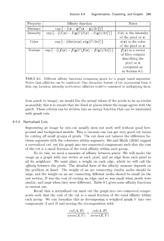
Property Affinity function Notes
(
)
t
Distance exp − (x − y) (x − y)/2σ 2 d
(
)
t
Intensity exp − (I(x) − I(y)) (I(x) − I(y))/2σ 2 I(x) is the intensity
I
of the pixel at x.
(
2 2 )
Color exp − dist(c(x), c(y)) /2σ c c(x) is the color
of the pixel at x.
(
)
t
Texture exp − (f(x) − f(y)) (f(x) − f(y))/2σ 2 f(x)is a vector
I
of filter outputs
describing the
pixel at x
computed as
in Section 6.1.
TABLE 9.1: Different affinity functions comparing pixels for a graph based segmenter.
Notice that affinities can be combined. One attractive feature of the exponential form is
that, say, location, intensity and texture affinities could be combined by multiplying them.

from patch to image), we would like the actual values of the pixels to be as similar
as possible; this is to ensure that we blend at places where the image agrees with the
patch. These criteria can be written into an energy function that can be minimized
with graph cuts.

9.4.4 Normalized Cuts
Segmenting an image by min-cut usually does not work well without good fore-
ground and background models. This is because one can get very good cut values
by cutting off small groups of pixels. The cut does not balance the difference be-
tween segments with the coherence within segments. Shi and Malik (2000) suggest
a normalized cut: cut the graph into two connected components such that the cost
of the cut is a small fraction of the total affinity within each group.
To do this, we need a measure of affinity between pixels. We will model the
image as a graph with one vertex at each pixel, and an edge from each pixel to
all its neighbors. We must place a weight on each edge, which we will call the
affinity between the pixels. The detailed form of the affinity measure depends on
theproblemathand. Theweightofanarc connecting similar nodes should be
large, and the weight on an arc connecting different nodes should be small (in the
last section, B was the cost of cutting an edge, and so was small when pixels were
similar, and large when they were different). Table 9.1 gives some affinity functions
in current use.
Recall that a normalized cut must cut the graph into two connected compo-
nents such that the cost of the cut is a small fraction of the total affinity within
each group. We can formalize this as decomposing a weighted graph V into two
components A and B and scoring the decomposition with
cut(A, B) cut(A, B)
+
assoc(A, V ) assoc(B, V )