Page 359 - Discrete Mathematics and Its Applications

338 5 / Induction and Recursion

INDUCTIVE STEP: The inductive hypothesis is the statement that P(j) is true for 12 ≤ j ≤ k,
where k is an integer with k ≥ 15. To complete the inductive step, we assume that we can form
postage of j cents, where 12 ≤ j ≤ k. We need to show that under the assumption that P(k + 1)
is true, we can also form postage of k + 1 cents. Using the inductive hypothesis, we can assume
that P(k − 3) is true because k − 3 ≥ 12, that is, we can form postage of k − 3 cents using
just 4-cent and 5-cent stamps. To form postage of k + 1 cents, we need only add another 4-cent
stamp to the stamps we used to form postage of k − 3 cents. That is, we have shown that if the
inductive hypothesis is true, then P(k + 1) is also true. This completes the inductive step.

Because we have completed the basis step and the inductive step of a strong induction proof,
we know by strong induction that P (n) is true for all integers n with n ≥ 12. That is, we know
that every postage of n cents, where n is at least 12, can be formed using 4-cent and 5-cent
stamps. This finishes the proof by strong induction.
(There are other ways to approach this problem besides those described here. Can you find
a solution that does not use mathematical induction?) ▲

Using Strong Induction in Computational Geometry

Our next example of strong induction will come from computational geometry, the part of
discrete mathematics that studies computational problems involving geometric objects. Compu-
tational geometry is used extensively in computer graphics, computer games, robotics, scientific
calculations, and a vast array of other areas. Before we can present this result, we introduce
some terminology, possibly familiar from earlier studies in geometry.
A polygon is a closed geometric figure consisting of a sequence of line segments
s 1 ,s 2 ,...,s n , called sides. Each pair of consecutive sides, s i and s i+1 , i = 1, 2,...,n − 1,
as well as the last side s n and the first side s 1 , of the polygon meet at a common endpoint,
called a vertex. A polygon is called simple if no two nonconsecutive sides intersect. Every sim-
ple polygon divides the plane into two regions: its interior, consisting of the points inside the
curve, and its exterior, consisting of the points outside the curve. This last fact is surprisingly
complicated to prove. It is a special case of the famous Jordan curve theorem, which tells us
that every simple curve divides the plane into two regions; see [Or00], for example.
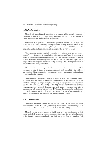
A polygon is called convex if every line segment connecting two points in the interior of the
polygon lies entirely inside the polygon. (A polygon that is not convex is said to be nonconvex.)
Figure 1 displays some polygons; polygons (a) and (b) are convex, but polygons (c) and (d) are
not.A diagonal of a simple polygon is a line segment connecting two nonconsecutive vertices of
the polygon, and a diagonal is called an interior diagonal if it lies entirely inside the polygon, ex-
cept for its endpoints. For example, in polygon (d), the line segment connecting a and f is an inte-
rior diagonal, but the line segment connecting a and d is a diagonal that is not an interior diagonal.
One of the most basic operations of computational geometry involves dividing a simple
polygon into triangles by adding nonintersecting diagonals.This process is called triangulation.
Note that a simple polygon can have many different triangulations, as shown in Figure 2. Perhaps
the most basic fact in computational geometry is that it is possible to triangulate every simple

a a g
a d a f
f
b
b e e
c d
af is an interior diagonal
b c c d b d c ad is not an interior diagonal
(a) (b) (c) (d)

FIGURE 1 Convex and Nonconvex Polygons.