Page 113 -

HAN 09-ch02-039-082-9780123814791

76 Chapter 2 Getting to Know Your Data 2011/6/1 3:15 Page 76 #38

(f )
where the indicator δ = 0 if either (1) x if or x jf is missing (i.e., there is no mea-
ij
surement of attribute f for object i or object j), or (2) x if = x jf = 0 and attribute
(f )
f is asymmetric binary; otherwise, δ = 1. The contribution of attribute f to the
ij
(f )
dissimilarity between i and j (i.e., d ) is computed dependent on its type:
ij
(f ) |x if −x jf |
If f is numeric: d = , where h runs over all nonmissing objects for
ij max h x hf −min h x hf
attribute f .
(f ) (f )
If f is nominal or binary: d = 0 if x if = x jf ; otherwise, d = 1.
ij ij
r if −1
If f is ordinal: compute the ranks r if and z if = , and treat z if as numeric.
M f −1
These steps are identical to what we have already seen for each of the individual
attribute types. The only difference is for numeric attributes, where we normalize so
that the values map to the interval [0.0, 1.0]. Thus, the dissimilarity between objects
can be computed even when the attributes describing the objects are of different
types.

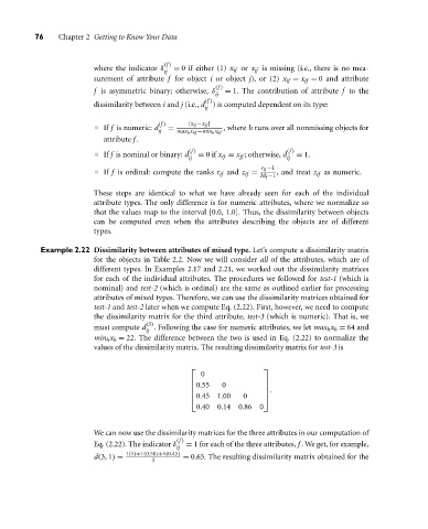
Example 2.22 Dissimilarity between attributes of mixed type. Let’s compute a dissimilarity matrix
for the objects in Table 2.2. Now we will consider all of the attributes, which are of
different types. In Examples 2.17 and 2.21, we worked out the dissimilarity matrices
for each of the individual attributes. The procedures we followed for test-1 (which is
nominal) and test-2 (which is ordinal) are the same as outlined earlier for processing
attributes of mixed types. Therefore, we can use the dissimilarity matrices obtained for
test-1 and test-2 later when we compute Eq. (2.22). First, however, we need to compute
the dissimilarity matrix for the third attribute, test-3 (which is numeric). That is, we
(3)
must compute d . Following the case for numeric attributes, we let max h x h = 64 and
ij
min h x h = 22. The difference between the two is used in Eq. (2.22) to normalize the
values of the dissimilarity matrix. The resulting dissimilarity matrix for test-3 is

 
0
0.55 0 

.


0.45 1.00 0 
0.40 0.14 0.86 0
We can now use the dissimilarity matrices for the three attributes in our computation of
(f )
Eq. (2.22). The indicator δ = 1 for each of the three attributes, f . We get, for example,
ij
d(3, 1) = 1(1)+1(0.50)+1(0.45) = 0.65. The resulting dissimilarity matrix obtained for the
3