Page 292 -

13-ch06-243-278-9780123814791
#13
3:20 Page 255
2011/6/1
HAN
6.2 Frequent Itemset Mining Methods 255

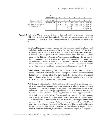
H 2
bucket address 0 1 2 3 4 5 6
Create hash table H 2 bucket count 2 2 4 2 2 4 4
using hash function bucket contents {I1, I4} {I1, I5} {I2, I3} {I2, I4} {I2, I5} {I1, I2} {I1, I3}
h(x, y) ((order of x) 10 {I3, I5} {I1, I5} {I2, I3} {I2, I4} {I2, I5} {I1, I2} {I1, I3}
(order of y)) mod 7 {I2, I3} {I1, I2} {I1, I3}
{I2, I3} {I1, I2} {I1, I3}

Figure 6.5 Hash table, H 2 , for candidate 2-itemsets. This hash table was generated by scanning
Table 6.1’s transactions while determining L 1 . If the minimum support count is, say, 3, then
the itemsets in buckets 0, 1, 3, and 4 cannot be frequent and so they should not be included
in C 2 .

Hash-based technique (hashing itemsets into corresponding buckets): A hash-based
technique can be used to reduce the size of the candidate k-itemsets, C k , for k > 1.
For example, when scanning each transaction in the database to generate the frequent
1-itemsets, L 1 , we can generate all the 2-itemsets for each transaction, hash (i.e., map)
them into the different buckets of a hash table structure, and increase the correspond-
ing bucket counts (Figure 6.5). A 2-itemset with a corresponding bucket count in the
hash table that is below the support threshold cannot be frequent and thus should
be removed from the candidate set. Such a hash-based technique may substantially
reduce the number of candidate k-itemsets examined (especially when k = 2).

Transaction reduction (reducing the number of transactions scanned in future itera-
tions): A transaction that does not contain any frequent k-itemsets cannot contain any
frequent (k + 1)-itemsets. Therefore, such a transaction can be marked or removed
from further consideration because subsequent database scans for j-itemsets, where
j > k, will not need to consider such a transaction.

Partitioning (partitioning the data to find candidate itemsets): A partitioning tech-
nique can be used that requires just two database scans to mine the frequent itemsets
(Figure 6.6). It consists of two phases. In phase I, the algorithm divides the trans-
actions of D into n nonoverlapping partitions. If the minimum relative support
threshold for transactions in D is min sup, then the minimum support count for a
partition is min sup × the number of transactions in that partition. For each partition,
all the local frequent itemsets (i.e., the itemsets frequent within the partition) are found.
A local frequent itemset may or may not be frequent with respect to the entire
database, D. However, any itemset that is potentially frequent with respect to D must
8
occur as a frequent itemset in at least one of the partitions. Therefore, all local frequent
itemsets are candidate itemsets with respect to D. The collection of frequent itemsets
from all partitions forms the global candidate itemsets with respect to D. In phase II,

8 The proof of this property is left as an exercise (see Exercise 6.3d).