Page 339 - Design and Operation of Heat Exchangers and their Networks

Dynamic analysis of heat exchangers and their networks 325

To solve Eqs. (7.1)–(7.5), we shall at first determine the mean temper-
atures t h , t c , and t w and the mean temperature differences Δt m,h and Δt m,c .
Different definitions of the mean temperatures and mean temperature dif-
ferences will yield different lumped parameter models.
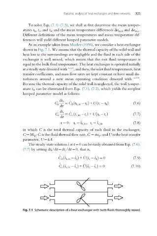
As an example taken from Mozley (1956), we consider a heat exchanger
shown in Fig. 7.1. We assume that the thermal capacity of the solid wall and
heat loss to the surroundings are negligible and the fluid in each side of the
exchanger is well mixed, which means that the exit fluid temperature is
equal to the bulk fluid temperature. The heat exchanger is operated initially
at a steady state denoted with “^”, and then, the inlet fluid temperatures, heat
transfer coefficients, and mass flow rates are kept constant or have small dis-
turbances around a new mean operating condition denoted with “¯”.
Because the thermal capacity of the solid wall is neglected, the wall temper-
ature t w can be eliminated from Eqs. (7.1), (7.2), which yields the simplest
lumped parameter model as follows:
dt h _
ð
ð
C h ¼ C h t h,in t h Þ + Ut c t h Þ (7.6)
dτ
dt c _
ð
ð
C c ¼ C c t c,in t c Þ + Ut h t c Þ (7.7)
dτ
(7.8)
τ ¼ 0 : t h ¼ ^ t h,in , t c ¼^ t c,in
in which C is the total thermal capacity of each fluid in the exchanger,
_
_
C¼Mc p ; C is the fluid thermal flow rate, C ¼ _mc p ; and U is the heat transfer
parameter, U¼kA.
The steady-state solution ^ t at τ¼0 can be easily obtained from Eqs. (7.6),
(7.7) by setting dt h /dτ¼dt c /dτ¼0, that is,
^
_ ^ t h,in ^ t h Þ + ^ U ^ t c ^ t h Þ ¼ 0
C h ð ð (7.9)
^
_ ^ t c,in ^ t c Þ + ^ U ^ t h ^ t c Þ ¼ 0
C c ð ð (7.10)

Fig. 7.1 Schematic description of a heat exchanger with both fluids thoroughly mixed.