Page 343 - Design and Operation of Heat Exchangers and their Networks

Dynamic analysis of heat exchangers and their networks 329

investigated the effects of the axial dispersion and heat conduction resis-
tances of tubes and shells on the dynamic behavior of heat exchangers
(Roetzel and Xuan, 1992b, 1993b). The numerical inverse algorithm
that they used is the Gaver-Stehfest algorithm (Stehfest, 1970; Jacquot
et al., 1983), which is valid only if the solution in the real-time domain
is continuous and monotone for τ>0. Luo (1998) suggested that the
numerical inverse Laplace transform with the FFT algorithm (Ichikawa
and Kishima, 1972) should be used for the general analysis of heat
exchanger dynamics.
From the earlier literature, we can see that the investigation on the
dynamic behavior of parallel-flow and counterflow heat exchangers were
limited to linear problems, that is, the temperature responses to arbitrary
inlet fluid temperature variations or step changes in mass flow rates. The
temperature responses to small disturbances in mass flow rates and heat trans-
fer coefficients were solved by Luo et al. (2003) by means of the linearization
treatment, Laplace transform, and numerical inverse algorithm with FFT. If
the disturbances are large or if there is a phase change in the heat exchanger,
then the problem would be strongly nonlinear, and the numerical method
should be used.
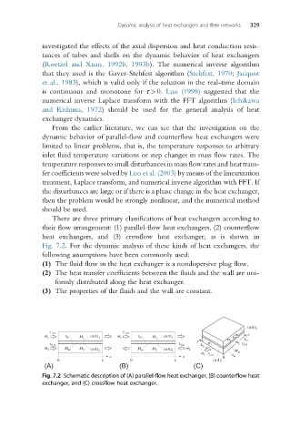
There are three primary classifications of heat exchangers according to
their flow arrangement: (1) parallel-flow heat exchangers, (2) counterflow
heat exchangers, and (3) crossflow heat exchanger, as is shown in
Fig. 7.2. For the dynamic analysis of these kinds of heat exchangers, the
following assumptions have been commonly used:
(1) The fluid flow in the heat exchanger is a nondispersive plug flow.
(2) The heat transfer coefficients between the fluids and the wall are uni-
formly distributed along the heat exchanger.
(3) The properties of the fluids and the wall are constant.

(aA) 2
t 1,in t 1,in x
˙ ˙
m 1 t w (aA) 1 m 1 t w (aA) 1
M 1 M 1
y M 2 ˙ L x
t 2,in t 2,in L y M 1 m 2 t 2,in
˙
m 2 M w M 2 m 2 ˙
(aA) 2 M w M 2 (aA) 2
˙ M w
m 1 t 1,in
x x 0 t w
0 L 0 L (aA) 1
(A) (B) (C)
Fig. 7.2 Schematic description of (A) parallel-flow heat exchanger, (B) counterflow heat
exchanger, and (C) crossflow heat exchanger.