Page 346 - Design and Operation of Heat Exchangers and their Networks

332 Design and operation of heat exchangers and their networks

In the literature, it is commonly assumed that the heat transfer coefficient
is a function of mass flow rates, for example,
α ¼ C _m n (7.44)
Therefore, only two disturbances are considered: disturbances in inlet fluid
temperatures and those in mass flow rates. This method is not general
because (1) the relationship between the heat transfer coefficient and
the mass flow rate cannot be universally expressed with Eq. (7.44) and (2)
the heat transfer coefficient can also be influenced by other factors. In the
present work, the heat transfer coefficient is taken as an independent distur-
bance. If the variation of the mass flow rate with time and the relationship
between the mass flow rate and the heat transfer coefficient are known, the
heat transfer coefficient is a known function of time.
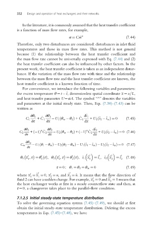
For convenience, we introduce the following variables and parameters:
the excess temperature θ ¼ t ^ t, dimensionless spatial coordinate x ¼ x=L,
and heat transfer parameter U¼αA. The symbol “^” denotes the variables
and parameters at the initial steady state. Then, Eqs. (7.38)–(7.43) can be
written as

∂θ 1 _ ∂θ 1 _ d^ t 1
^ ð
ð
C 1 + C 1 U 1 θ w θ 1 Þ + C 1 + U 1 t 1 ^ t w Þ ¼ 0 (7.45)
∂τ ∂x dx
∂θ 2 n _ ∂θ 2 n _ d^ t 2
^ ð
ð
ð
C 2 + 1Þ C 2 U 2 θ w θ 2 Þ + 1ð Þ C 2 + U 2 t 2 ^ t w Þ ¼ 0 (7.46)
∂τ ∂x dx
∂θ w
^ ð
^ ð
ð
ð
C w U 1 θ 1 θ w Þ U 2 θ 2 θ w Þ U 1 t 1 ^ t w Þ U 2 t 2 ^ t w Þ ¼ 0 (7.47)
∂τ

0 0
^
^
0
0
0
0
0
θ 1 x , τ ¼ θ τðÞ, θ 2 x , τ ¼ θ τðÞ, ^ t 1 x ¼^ t , ^ t 2 x ¼^ t 0 (7.48)
1 1 2 2 1 1 2 2
τ ¼ 0 : θ 1 ¼ θ 2 ¼ θ w ¼ 0 (7.49)
0 0
0
0
where x ¼ ^ x ¼ 0, x ¼ n, and ^ x ¼ ^n. It means that the flow direction of
1 1 2 2 0
0
fluid 2 can have a sudden change. For example, x ¼ 0 and ^ x ¼ 1 means that
2 2
the heat exchanger works at first in a steady counterflow state and then, at
τ¼0, a changeover takes place to the parallel-flow condition.
7.1.2.5 Initial steady-state temperature distribution
To solve the governing equation system (7.45)–(7.49), we should at first
obtain the initial steady-state temperature distribution. Deleting the excess
temperatures in Eqs. (7.45)–(7.48), we have