Page 422 - Design and Operation of Heat Exchangers and their Networks

Experimental methods for thermal performance of heat exchangers 405

The heat flux is kept at a constant value by carefully regulating the hot water
temperature. Its value should be carefully estimated so that the temperature
change of the hot water from its inlet to outlet is about 4K under the max-
imum flow rate of the hot water. Applying the original Wilson plot method,
we can determine the value of C i , and therefore, the correlation for convec-
tive heat transfer coefficient inside the tube α i is obtained.
In the second test set, other six or more test runs are carried out under the
specified heat fluxes whose logarithmic values are equally divided. The
change of the heat flux is realized by varying the hot water flow rate but
keeping the inlet temperature of the hot water unchanged. With known
α i,j and the measured values of (kA) j , the evaporation heat transfer coeffi-
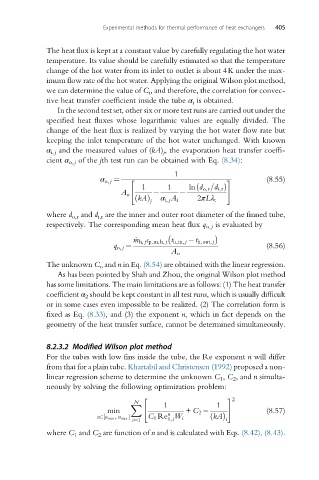
cient α o,j of the jth test run can be obtained with Eq. (8.34):

1
α o, j ¼ " # (8.55)
1 1 ln d o,r =d i,r Þ
ð
A o
ð kAÞ α i, j A i 2πLλ t
j
where d o,r and d i,r are the inner and outer root diameter of the finned tube,
respectively. The corresponding mean heat flux q o,j is evaluated by

_ m h, j c p,m,h, j t h,in, j t h,out, j
q o, j ¼ (8.56)
A o
The unknown C o and n in Eq. (8.54) are obtained with the linear regression.
As has been pointed by Shah and Zhou, the original Wilson plot method
has some limitations. The main limitations are as follows: (1) The heat transfer
coefficient α 2 should be kept constant in all test runs, which is usually difficult
or in some cases even impossible to be realized. (2) The correlation form is
fixed as Eq. (8.33), and (3) the exponent n, which in fact depends on the
geometry of the heat transfer surface, cannot be determined simultaneously.

8.2.3.2 Modified Wilson plot method
For the tubes with low fins inside the tube, the Re exponent n will differ
from that for a plain tube. Khartabil and Christensen (1992) proposed a non-
linear regression scheme to determine the unknown C 1 , C 2 , and n simulta-
neously by solving the following optimization problem:
" # 2
N
X 1 1
min + C 2 (8.57)
n
n2 n min, n max Š C 1 Re W i ð kAÞ i
½
1,i
i¼1
where C 1 and C 2 are function of n and is calculated with Eqs. (8.42), (8.43).