Page 418 - Design and Operation of Heat Exchangers and their Networks

Experimental methods for thermal performance of heat exchangers 401

in which n and m are constants taken from the literature, for example, from
the Dittus-Boelter correlation (Dittus and Boelter, 1930) with n¼0.8,
m¼0.4 for heating, and m¼0.3 for cooling. We also assume that the heat
transfer coefficients of the two fluids are uniform along their flow directions,
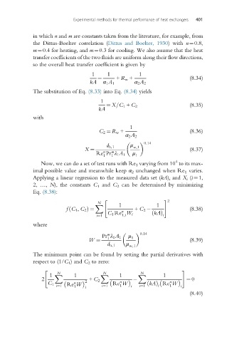
so the overall heat transfer coefficient is given by
1 1 1
¼ + R w + (8.34)
kA α 1 A 1 α 2 A 2
The substitution of Eq. (8.33) into Eq. (8.34) yields
1
¼ X=C 1 + C 2 (8.35)
kA
with

1
C 2 ¼ R w + (8.36)
α 2 A 2
μ 0:14
d h,1 w,1
X ¼ (8.37)
n m μ
Re Pr λ 1 A 1 1
1 1
4
Now, we can do a set of test runs with Re 1 varying from 10 to its max-
imal possible value and meanwhile keep α 2 unchanged when Re 1 varies.
Applying a linear regression to the measured data set (kA) i and X i (i¼1,
2, …, N), the constants C 1 and C 2 can be determined by minimizing
Eq. (8.38):
" # 2
N
X 1 1
ð
fC 1 , C 2 Þ ¼ + C 2 (8.38)
n
C 1 Re W i ð kAÞ
i¼1 1,i i
where
m μ 0:14
Pr λ 1 A 1 1
1
W ¼ (8.39)
d h,1 μ w,1
The minimum point can be found by setting the partial derivatives with
respect to (1/C 1 ) and C 2 to zero:
" #
N
N
N
1 X 1 X 1 X 1
2 + C 2 n n ¼ 0
2
i¼1 Re W i i¼1 1 i i¼1 i 1 i
C 1 n Re W ð kAÞ Re W
1
(8.40)