Page 351 - Design of Simple and Robust Process Plants

8.4 Control Design 337
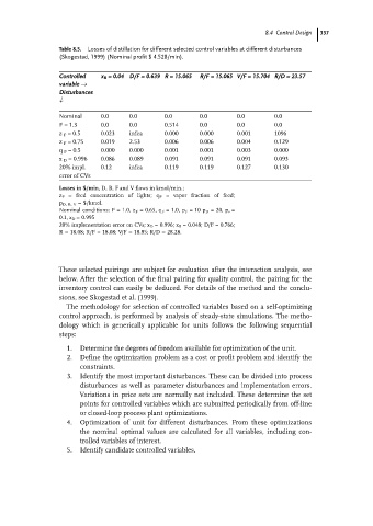
Table 8.5. Losses of distillation for different selected control variables at different disturbances
(Skogestad, 1999) (Nominal profit $ 4.528/min).

Controlled x B = 0.04 D/F = 0.639 R = 15.065 R/F = 15.065 V/F = 15.704 R/D = 23.57
variable ®
Disturbances
¯
Nominal 0.0 0.0 0.0 0.0 0.0 0.0
F = 1.3 0.0 0.0 0.514 0.0 0.0 0.0
z F = 0.5 0.023 infea 0.000 0.000 0.001 1096
z F = 0.75 0.019 2.53 0.006 0.006 0.004 0.129
q F = 0.5 0.000 0.000 0.001 0.001 0.003 0.000
x D = 0.996 0.086 0.089 0.091 0.091 0.091 0.093
20% impl. 0.12 infea 0.119 0.119 0.127 0.130
error of CVs
Losses in $/min, D, B, F and V flows in kmol/min.;
z F = feed concentration of lights; q F = vapor fraction of feed;
p D, B, V = $/kmol.
Nominal conditions: F = 1.0, z F = 0.65, q F = 1.0, p F =10 p D = 20, p v =
0.1, x D = 0.995
20% implementation error on CVs; x D = 0.996; x B = 0.048; D/F = 0.766;
R = 18.08; R/F = 18.08; V/F = 18.85; R/D = 28.28.

These selected pairings are subject for evaluation after the interaction analysis, see
below. After the selection of the final pairing for quality control, the pairing for the
inventory control can easily be deduced. For details of the method and the conclu-
sions, see Skogestad et al. (1999).
The methodology for selection of controlled variables based on a self-optimizing
control approach, is performed by analysis of steady-state simulations. The metho-
dology which is generically applicable for units follows the following sequential
steps:

1. Determine the degrees of freedom available for optimization of the unit.
2. Define the optimization problem as a cost or profit problem and identify the
constraints.
3. Identify the most important disturbances. These can be divided into process
disturbances as well as parameter disturbances and implementation errors.
Variations in price sets are normally not included. These determine the set
points for controlled variables which are submitted periodically from off-line
or closed-loop process plant optimizations.
4. Optimization of unit for different disturbances. From these optimizations
the nominal optimal values are calculated for all variables, including con-
trolled variables of interest.
5. Identify candidate controlled variables.