Page 157 - Designing Autonomous Mobile Robots : Inside the Mindo f an Intellegent Machine

Chapter 10

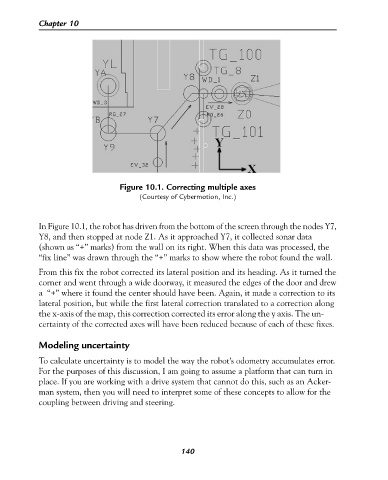
Figure 10.1. Correcting multiple axes
(Courtesy of Cybermotion, Inc.)

In Figure 10.1, the robot has driven from the bottom of the screen through the nodes Y7,
Y8, and then stopped at node Z1. As it approached Y7, it collected sonar data
(shown as “+” marks) from the wall on its right. When this data was processed, the
“fix line” was drawn through the “+” marks to show where the robot found the wall.

From this fix the robot corrected its lateral position and its heading. As it turned the
corner and went through a wide doorway, it measured the edges of the door and drew
a “+” where it found the center should have been. Again, it made a correction to its
lateral position, but while the first lateral correction translated to a correction along
the x-axis of the map, this correction corrected its error along the y axis. The un-
certainty of the corrected axes will have been reduced because of each of these fixes.

Modeling uncertainty

To calculate uncertainty is to model the way the robot’s odometry accumulates error.
For the purposes of this discussion, I am going to assume a platform that can turn in
place. If you are working with a drive system that cannot do this, such as an Acker-
man system, then you will need to interpret some of these concepts to allow for the
coupling between driving and steering.

140