Page 189 - Determinants and Their Applications in Mathematical Physics

174 5. Further Determinant Theory

5.1.3 Orthogonal Polynomials
Determinants which represent orthogonal polynomials (Appendix A.5)
have been constructed using various methods by Pandres, R¨osler, Yahya,
Stein et al., Schleusner, and Singhal, Frost and Sackfield and others. The
following method applies the Rodrigues formulas for the polynomials.
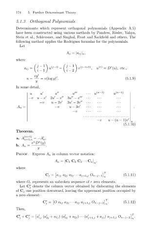
Let
A n = |a ij | n ,

where

j − 1 (j−i) j − 1 (j−i+1) (r)
a ij = u − v , u = D (u), etc.,
r
i − 1 i − 2
vy

u = = v(log y) . (5.1.9)
y
In some detail,
u u u u ··· u (n−2) u (n−1)

−v u − v 2u − v 3u − v ··· ··· ···

−v u − 2v 3u − 3v ··· ··· ···

−v u − 3v ··· ··· ··· .

A n =
−v ··· ··· ···

............................
−v u − (n − 1)v

n
(5.1.10)
Theorem.
(n+1)
a. A = −A ,

n
n+1,n
v D (y)
n
n
b. A n = .
y
Proof. Express A n in column vector notation:

A n = C 1 C 2 C 3 ··· C n ,

n
where

T
C j = a 1j a 2j a 3j ··· a j+1,j O n−j−1 (5.1.11)
n
where O r represents an unbroken sequence of r zero elements.
Let C denote the column vector obtained by dislocating the elements
∗
j
of C j one position downward, leaving the uppermost position occupied by
a zero element:

∗ T
C = Oa 1j a 2j ··· a jj a j+1,j O n−j−2 . (5.1.12)
j
n
Then,
T

C + C = a (a + a 1j )(a + a 2j ) ··· (a + a jj ) a j+1,j O n−j−2 .
∗
j j 1j 2j 3j j+1,j
n