Page 187 - Distillation theory

P1: JPJ/FFX P2: FCH/FFX QC: FCH/FFX T1: FCH
0521820928c05 CB644-Petlyuk-v1 June 11, 2004 20:15

5.6 Conditions of Section Trajectories Joining and Methods 161

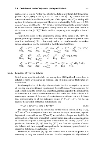
section); (2) at joining “at the type of intermediate split without distributed com-
2
+
ponents” 1,2 : 3,4 (Fig. 5.35a; x D = 0.4, x f −1 lies at line S − N , zone of constant
r r
concentrations is located in the middle part of the top section); (3) at joining with
optimal distribution of component 2 between products (Fig. 5.35c; x D2 = 0, 268,
2
+
+
x f ≡ N s , x f −1 lies at line S − N , zones of constant concentrations are available
r r
in both sections: in the middle part of the top section and in feed cross-section in
the bottom section, [L/V] min is the smallest comparing with any splits at items 1
r
and 2).
Figure 5.35d shows for this example the change of the value of (L/V) min , de-
r
pending on the parameter x D2 (the first two stages of general algorithm were
used for calculations). The column trajectories, the calculation direction taken
into consideration, may be presented in the following brief form:
(2) 1(2) 2(3) (4) (4) 1(3) (3)
x → S → S → x ⇓⇒ x ← S ← x (Fig. 5.35a)
D r r f −1 f s B
Reg Reg t Reg t min,R sh,R Reg t Reg
D r r Reg Reg s B
sep,r sep,s
(2) 1(2) (4) (4) 1(3) (3)
x → S → x ⇓⇒ x ← S ← x (Fig. 5.35b)
D r f −1 f s B
Reg Reg t sh,R + Reg t Reg
D r Reg N s s B
sep,r
(2) 1(2) 2(3) (4) (4) 1(3) (3)
x → S → S → x ⇓⇒ x ← S ← x (Fig. 5.35c)
D r r f −1 f s B
Reg Reg t Reg t min,R + Reg t Reg
D r r Reg N s s B
sep,r
5.6.6. Equations of Thermal Balance
Stated above algorithms include two assumptions: (1) liquid and vapor flows in
column sections are accepted as constant, and (2) it is accepted that plates are
equilibrium.
Small complication of the algorithms excludes the first assumption by means
of entering into algorithms of equations of thermal balance. These equations for
each section should be constructed at contour, embracing part of the column from
cross-section in a zone of constant concentration to the end of the column. It is
necessary to examine all the zones of constant concentrations – real and fictitious
2
3
1
+
(i.e., corresponding to all the stationary points:S , S , S ...N ). For the top
section, the equation of thermal balance looks like
st st
st
st
top top
V H + L h = L h + V top H top (5.21)
r r r r r r r r
The similar equation can be constructed for the bottom section. In Eq. (5.21),
top top
H r and h r are enthalpies of liquid and vapor at the top of the column, depend-
st
st
ing on their compositions, and H and h are enthalpies of vapor and liquid in the
r r
cross-section of the zone of constant concentrations, depending on composition
top
in the stationary point. Knowing these compositions and setting (L/V) r ,itis
st
possible to determine (L/V) from Eq. (5.21) and from the equation of mate-
r
rial balance and then to specify composition in the stationary point, located at
st
reversible distillation trajectory for (L/V) .
r
st
Therefore, to determine (L/V) and compositions in stationary points, it is
r
necessary to carry out several iterations. In other respects, the algorithms of