Page 268 - Distillation theory

P1: JPJ/FFX P2: JMT/FFX QC: FCH/FFX T1: FCH
0521820928c07 CB644-Petlyuk-v1 June 11, 2004 20:18

242 Trajectories of the Finite Columns and Their Design Calculation

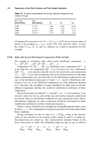
Table 7.2. Product concentration of non-key impurity component and
number of trays

η D = η B , x D4 ,
mol. fraction mol. fraction N r N s N tot
0.999 7.7·10 –8 7.06 14.29 21.35
0.990 3.7·10 –5 3.68 7.63 11.31
0.980 2.4·10 –4 2.69 5.68 8.37
0.950 1.8·10 –3 1.75 3.22 4.97

(2)-heptane(3)-octane(4) at (L/V) r = 0.5, x D,2 = 0.336 and at several values of
purity of the products η D = η B = 0.999, 0.99, 0.98, and 0.95. Table 7.2 gives
the values of x D,4 , N r , N s , and N tot obtained as a result of calculation for this
example.

7.3.4. Splits with Several Distributed Components: Preferred Split
We examine in conclusion splits with several distributed components −1,
2,..., k dist , k dist ,..., k dist : k dist , k dist ,..., k dist ,... n.
1 2 m 1 2 m
Components k dist , k dist ,..., k dist are distributed ones, component (k dist − 1)
1 2 m 1
is the light key one, component (k dist + 1) is the heavy key one, components
m
(k dist + 2),..., n are non-key impurity ones in the top product, and components
m
1, 2 ..., (k dist − 2) are non-key impurity ones in the bottom product. For the splits
1
under consideration, one can arbitrarily set the distribution coefficient for only
one of the distributed components β (minβ< β< maxβ). Distribution coef-
ficients of the rest of the distributed components are some unknown functions
of β. Therefore, the algorithm of design calculation for splits with several dis-
tributed components includes the search for distribution coefficients of these
components.
The preferred split, for which k dist = 2 and k dist = (n − 1), is an exclusion. Com-
1 m
ponents 1 and n are the key ones in this case, and non-key impurity components
are absent. Only one distribution coefficient for one component can be chosen.
Distribution coefficients for other components should be determined by phase
equilibrium coefficients of all the components in point x F .
Points x D and x B should lie in the straight line passing through the liquid–vapor
tie-line x F → y F . The compositions of separation products can be determined from
these conditions.
Design calculation for the set value of σ = R/R min comes to the determi-
nation of tray numbers in the sections of the column N r and N s at which sec-
tion trajectories are joined (i.e., the componentwise material balance in the
feed cross-section is valid). The distillation trajectory may be put as follows:

1 1
x D → qS → x f −1 ⇒⇓ x f ← qS ← x B .
s
r
Reg D Reg t r Reg rev Reg rev Reg t s Reg B