Page 223 - Distributed model predictive control for plant-wide systems

Cooperative Distributed Predictive Control with Constraints 197

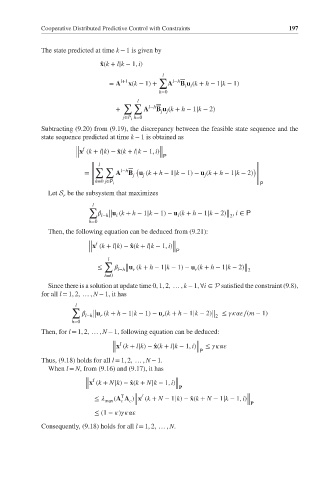
The state predicted at time k − 1 is given by
̂ x(k + l|k − 1, i)
l
∑ l−h
l+1
= A x(k − 1)+ A B u (k + h − 1|k − 1)
i i
h=0
l
∑ ∑ l−h
+ A B u (k + h − 1|k − 2)
j j
j∈P i h=0
Subtracting (9.20) from (9.19), the discrepancy between the feasible state sequence and the
state sequence predicted at time k − 1 is obtained as
‖ f ‖
‖x (k + l|k) − ̂ x(k + l|k − 1, i)‖
‖ ‖P
‖ l ‖
‖∑ ∑ l−h ( )‖
= ‖ A B u (k + h − 1|k − 1) − u (k + h − 1|k − 2) ‖
j
j
j
‖ ‖
‖ ‖
h=0 j∈P i ‖P
‖
Let S be the subsystem that maximizes
r
l
∑
u (k + h − 1|k − 1) − u (k + h − 1|k − 2) , i ∈ P
‖
l−h‖ i i ‖
‖2
h=0
Then, the following equation can be deduced from (9.21):
‖ f ‖
‖x (k + l|k) − ̂ x(k + l|k − 1, i)‖
‖ ‖P
l
∑
u (k + h − 1|k − 1) − u (k + h − 1|k − 2)
≤ l−h‖ r r ‖
‖
‖2
h=0
Since there is a solution at update time 0, 1, 2, … , k − 1, ∀i ∈ P satisfied the constraint (9.8),
for all l = 1, 2, … , N − 1, it has
l
∑
u (k + h − 1|k − 1) − u (k + h − 1|k − 2)
l−h‖ r r ‖ ≤ ∕(m − 1)
‖
‖2
h=0
Then, for l = 1, 2, … , N − 1, following equation can be deduced:
‖ f ‖
‖x (k + l|k) − ̂ x(k + l|k − 1, i)‖ ≤
‖ ‖P
Thus, (9.18) holds for all l = 1, 2, … , N − 1.
When l = N, from (9.16) and (9.17), it has
‖ f ‖
‖x (k + N|k) − ̂ x(k + N|k − 1, i)‖
‖ ‖P
T ‖ f ‖
≤ (A A )‖x (k + N − 1|k) − ̂ x(k + N − 1|k − 1, i)‖
max c c
‖ ‖P
≤ (1 − )
Consequently, (9.18) holds for all l = 1, 2, … , N.