Page 96 - Distributed model predictive control for plant-wide systems

70 Distributed Model Predictive Control for Plant-Wide Systems

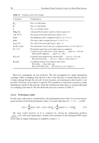
Table 5.1 Notations used in this chapter
5 Notations 6 Explanations

0 a × b The a × b null matrix
0 a The a × a null matrix
I a The a × a identity matrix
diag {A} A diagonal block matrix made by a blocks equal to A
a
T
2
‖v‖ ≜ v v The square of the norm induced by matrix v ⪰ 0.
̂ x(l|h) The prediction of x(l) computed at time h; l, h ∈ P, h < l
u(l|h) The value of u(l) computed at time h; l, h ∈ P, h < l
Δu ∈ ℝ n u i The control increment Δu ≜ u (k) − u (k − 1)
i i i i
ˆ w (l|h), ̂ v (l|h) The estimations of w (l)and v (l) computed at time h, l, h ∈ P and h < l
i i i i
Y ∈ ℝ n y i The desired output that can be either known or predicted
d
i
A stacked vector made by the vectors Δu (k|k), … , Δu (k + p − 1|k)and
i i
ΔU (k, p|k) ≜ {Δu (k|k), … , Δu (k + p − 1|k)}
i i i
X (l, p|h) A stacked vector made by the vectors x (l|h), … , x (l + p − 1|h), and
i i i
T
T
X (l, p|h) ≜ [x (l|h), … , x (l + p − 1|h)], p, l, h ∈ ℕ and h < l
i i i
X(l, p|h) A complete stacked vector made by the vectors
X (k, m|h), … , X (k, m|h), and
1
n
T
T
X(l, p|h) ≜ [X (l, p|h), … , X (l, p|h)], p, l, h ∈ ℕ and h < l
1 i
These two assumptions are not restrictive. The first assumption of a single information
exchange within a sampling time interval is due to the necessity of minimizing the amount
of data exchange through the network. In real situations, an instantaneous data transfer is not
possible. Therefore, the unit delay is required. This hypothesis is equivalent to assume a simple
deterministic model of the network, where the transmission time delay is constant and equal
to a sampling time interval. We also define the necessary notation in Table 5.1.
5.2.2.1 Performance Index
For the large-scale system, considered here, the global performance index (5.4) can be decom-
posed in terms of the local performance index J for each subsystem S , i = 1, 2, … , m [90]
i
i
P M
∑ d 2 ∑ 2
J (k)= + (5.5)
i
i
i ‖̂ y (k + l|k)− y (k + l|k)‖ Q i ‖Δu (k + l − 1|k)‖ R i
i
l=1 l=1
The local control decision of S is computed by solving the optimization problem
i
min J (k) with local input/output variables and constraints in the distributed MPC based
i
ΔU(k, M|k)
on the state (or input) estimations of neighbors at time k − 1.