Page 36 - Dynamic Loading and Design of Structures

Page 23

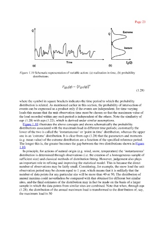
Figure 1.10 Schematic representation of variable action: (a) realization in time, (b) probability
distributions.

(1.28)

where the symbol in square brackets indicates the time period to which the probability
distribution is related. As mentioned earlier in this section, the probability of intersection of
events can be expressed as a product only if the events are independent; for time varying
loads this means that the unit observation time must be chosen so that the maximum value of
the load recorded within any such period is independent of the others. Note the similarity of
eqn (1.28) with eqn (1.22), which is derived under similar assumptions.
Figure 1.10 illustrates the above concepts and shows schematically the probability
distributions associated with the maximum load in different time periods; customarily the
lower of the two is called the ‘instantaneous’ or ‘point in time’ distribution, whereas the upper
one is an ‘extreme’ distribution. It is clear from eqn (1.28) that the parameters and moments
(e.g. mean value) of the extreme distribution are a function of the specified reference period.
The longer this is, the greater becomes the gap between the two distributions shown in Figure
1.10.
In principle, for actions of natural origin (e.g. wind, snow, temperature) the ‘instantaneous’
distribution is determined through observations (i.e. the creation of a homogeneous sample of
sufficient size) and classical methods of distribution fitting. However, judgement also plays
an important role in refining and improving the statistical model. This is because the direct
number of observations may be fairly small. Considering, for example, the snow load the unit
observation period may be chosen equal to 1 year, which means that it is unlikely that the
number of data points for any particular site will be more than 40 or 50, The distribution of
annual maxima could nevertheless be compared with that obtained for different but similar
sites, and the final estimates of the distribution may in fact be made on the basis of a larger
sample in which the data points from similar sites are combined. Note that when, through eqn
(1.28), the distribution of the annual maximum load is transformed to the distribution of, say,
the maximum load in 50