Page 37 - Dynamics and Control of Nuclear Reactors

28 CHAPTER 3 The point reactor kinetics equations

The transfer function can be recast to give per cent power deviation per cent of reac-
tivity as follows:
β
δ%P Λ
δc ¼ 0 β i 1 (3.35)
X 6 Λ
s 1+ C
B
@ A
ð
i¼1 s + λ i Þ
This form will be useful in subsequent discussions about reactor frequency response.
The transfer function for the model with a single group of delayed neutrons is.
β
δP per cent powerÞ Λ ð s + λÞ
ð
¼ (3.36)
δρ centÞ β
ð
ss + λ +
Λ
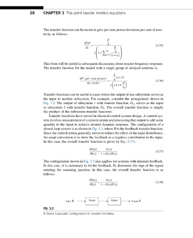
Transfer functions can be useful in cases where the output of one subsystem serves as
the input to another subsystem. For example, consider the arrangement shown in
Fig. 3.2. The output of subsystem 1 with transfer function, G 1 , serves as the input
to subsystem 2 with transfer function, G 2 . The overall transfer function is simply
the product of the subsystem transfer functions.
Transfer functions have served in classical control system design. A control sys-
tem involves measurement of a system output and processing that output to add some
quantity to the input to achieve desired dynamic response. The configuration of a
closed-loop system is as shown in Fig. 3.3, where H is the feedback transfer function.
Since the control action generally serves to reduce the effect of the input disturbance,
the usual convention is to show the feedback as a negative contribution to the input.
In this case, the overall transfer function is given by Eq. (3.37).

δOsðÞ GsðÞ
¼ (3.37)
δIsðÞ 1+ GsðÞHsðÞ
The configuration shown in Fig. 3.3 also applies for systems with inherent feedback.
In this case, it is customary to let the feedback, H, determine the sign of the signal
entering the summing junction. In this case, the overall transfer function is as
follows:

δOsðÞ GsðÞ
¼ (3.38)
δIsðÞ 1 GsðÞHsðÞ

Input X G1(s) G2(s) Output Y
FIG. 3.2
A Series (cascade) configuration of transfer functions.