Page 43 - Dynamics and Control of Nuclear Reactors

34 CHAPTER 4 Solutions of the point reactor kinetics equations

Available numerical methods can handle all of the model categories. The soft-
ware packages commonly require the model to be expressed as a set of coupled,
first-order differential equations (like we have seen for the point reactor kinetics
equations). These software packages require a model with n first-order differential
equations to be expressed as follows:
dx 1
¼ a 11 x 1 + a 12 x 2 + ⋯a 1n x n + f 1 (4.1)
dt

dx 2
¼ a 21 x 1 + a 22 x 2 + ⋯a 2n x n + f 2 (4.2)
dt
dx n
¼ a n1 x 1 + a n2 x 2 + ⋯a nn x n + f n (4.3)
dt
where, x i ¼ a dependent variable (i ¼ 1, 2, …,n), a ij ¼ a constant coefficient (i ¼ 1,
2, …,n; j ¼ 1, 2, …,n),f i ¼ a forcing function.
In matrix notation,
dX
¼ AX + f (4.4)
dt
X is (n 1) state vector, f is a (n 1) vector of forcing terms, and A is the (n n)
“system matrix” containing the system parameters. A model with n equations is
called an n-th order state variable model. The formulation in Eq. (4.4) is often called
the state-space representation of system dynamics. This representation, in general,
can also involve nonlinear functions of the state variables by adding a vector of non-
linear terms, g(X). See Appendix F for a description of state variable models.
Implementation requires supplying values for the elements in the A matrix and f
vector to appropriate software.
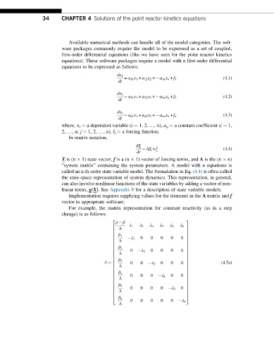
For example, the matrix representation for constant reactivity (as in a step
change) is as follows:
ρ β
2 3
Λ λ 1 λ 2 λ 3 λ 4 λ 5 λ 6
6 7
6 7
6 β 7
6 1 0 0 0 0 7
Λ
6 λ 1 0 7
6 7
β
6 7
6 2 7
6 0 λ 2 0 0 0 0 7
Λ
6 7
6 7
β
6 7
6 3 0 0 0 0 7 (4.5a)
Λ
A ¼ 6 λ 3 0 7
6 7
6 7
β
6 7
6 4 0 0 0 0 7
Λ
6 λ 4 0 7
6 7
β
6 7
6 5 7
Λ
6 0 0 0 0 λ 5 0 7
6 7
6 7
4 β 6 5
Λ 0 0 0 0 0 λ 6