Page 51 - Dynamics of Mechanical Systems

0593_C02_fm Page 32 Monday, May 6, 2002 1:46 PM

32 Dynamics of Mechanical Systems

A D D ⊥
D
ll
D
n
A n
A

θ θ

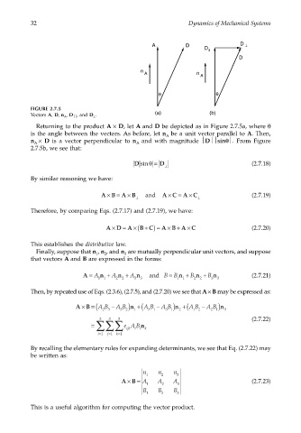
FIGURE 2.7.5
Vectors A, D, n A , D  , and D ⊥ . (a) (b)
Returning to the product A × D, let A and D be depicted as in Figure 2.7.5a, where θ
is the angle between the vectors. As before, let n be a unit vector parallel to A. Then,
A
n × D is a vector perpendicular to n and with magnitude Dsinθ. From Figure
A
A
2.7.5b, we see that:
D sinθ= D ⊥ (2.7.18)

By similar reasoning we have:

=
×
×
×
×
AB AB ⊥ and A C = A C ⊥ (2.7.19)
Therefore, by comparing Eqs. (2.7.17) and (2.7.19), we have:
+
×
×
×
+
AD = A ×( B C) = A B A C (2.7.20)
This establishes the distributive law.
Finally, suppose that n , n , and n are mutually perpendicular unit vectors, and suppose
1
3
2
that vectors A and B are expressed in the forms:
A = A n + A n + A n and B = B n + B n + B n (2.7.21)
1 1 2 2 3 3 1 1 2 2 3 3
Then, by repeated use of Eqs. (2.3.6), (2.7.5), and (2.7.20) we see that A × B may be expressed as:
×
AB = (AB − AB n ) +(AB − AB n ) +(A B − AB n )
23 3 2 1 3 1 3 1 2 1 2 2 1 3
3
3
3
= ∑ ∑ ∑ ijk ii n k (2.7.22)
eA B
= i 1 = j 1 k =1
By recalling the elementary rules for expanding determinants, we see that Eq. (2.7.22) may
be written as:

n n n
1 2 3
×
AB = A A A (2.7.23)
1 2 3
B B B
1 2 3
This is a useful algorithm for computing the vector product.